The Wealth Delta Tax: Taxpayer Welfare Comparison Across Tax Systems at Revenue Equivalence
Wealth Delta Tax, welfare comparison, Domar-Musgrave, capital gains tax lock-in, return heterogeneity, revenue equivalence
Revision History
| Revision | Date | Details |
|---|---|---|
| 0.01 | 13 September 2026 | Initial scaffold. |
| 0.02 | 16 September 2026 | Verbal compression |
| 0.03 | 16 September 2026 | Epistemic tightening: Arachi claim bounded to loss-year component with entry-margin qualification; P(locked in) decomposition relabelled to distinguish market preference from CGT-induced non-switching; T≥8 plateau reframed as realisation-induced portfolio persistence; SRR claim corrected to bound taxpayer-level exposure rather than eliminating solvency risk; 479× and income tax concentration figures qualified as model-simulated; welfare object taxonomy (CEW, incidence, concentration) distinguished in §6.1; asymmetric CGT/WDT treatment made prominent in §2.4; burden-of-consideration conclusion reframed analytically; incidence ≠ welfare progressivity distinction added to §4.3.4; horizon choice defended in §2.1; §7.4 TODO resolved — N=73 run committed to WFR.A §F. |
Abstract
This paper compares six tax systems — flat-rate symmetric WDT, progressive symmetric WDT, income tax, capital gains tax, stock wealth tax, and consumption tax — at genuine revenue equivalence (E[T] = 2% of \(W_0\)), using certainty-equivalent welfare against a common no-tax benchmark. Distortions are admitted one at a time in a controlled sequence, so welfare differences can be attributed to specific mechanisms rather than to bundled effects.
The paper closes three confirmed literature gaps. It formally extends the Domar-Musgrave risk-sharing framework to a progressive delta base and quantifies the three complications this introduces under a logistic rate schedule — all second-order at canonical parameters. It positions the delta base in a welfare comparison alongside the standard candidates, tested against the same empirical return distribution at revenue equivalence. And it traces the concentration path of persistent Fagereng-style return heterogeneity under each tax base over a 30-year horizon.
Three main results follow. First, a controlled baseline with all distortions suppressed shows the flat WDT leading income tax and CGT by 17.4 basis points — a small advantage establishing fair ground, not a knockout. Second, once portfolio choice is endogenous, CGT’s realisation lock-in imposes a welfare cost of 141–143 basis points at plausible UK parameters, approximately 82 times the baseline difference between systems; this cost is eliminated by construction under the WDT because the delta base does not make the switching decision tax-relevant. Third, stock wealth and consumption taxes allow the Fagereng return differential to compound into 479-fold Great/Poor wealth concentration at the 30-year horizon, versus 286–288-fold for WDT variants and 320-fold for income tax; the relevant axis is accrual basis versus stock base, not flat versus progressive rate.
The paper applies a three-category epistemic taxonomy distinguishing welfare costs of existing systems (Category 1), structural properties of the WDT (Category 2), and prospective implementation costs whose magnitude is unknown (Category 3). The welfare case for the WDT rests on Categories 1 and 2 alone; Category 3 costs are named and passed to the companion paper EVAL for break-even analysis.
Glossary
Certainty-equivalent welfare (CEW): The proportional change in consumption under a no-tax counterfactual that would make an agent indifferent to the taxed system. Negative values indicate a welfare cost relative to the no-tax benchmark.
Delta base: The annual change in an individual’s net worth, net of a cost-of-capital allowance, used as the tax base under the Wealth Delta Tax.
Domar-Musgrave (D-M) property: The result that a proportional tax with full symmetric loss offsets contracts the agent’s net return distribution without altering relative risk rankings, leaving the risk-taking incentive intact.
Lifetime contribution envelope: The mechanism bounding cumulative refunds at cumulative taxes paid by each taxpayer to date, preventing the symmetric refund from operating as open-ended public insurance.
Lock-in distortion: The welfare cost arising when a capital gains tax creates a switching wedge between the gross return differential and the after-tax return from realising a position, causing the taxpayer to remain in an inferior asset.
Long-run reserve (LRR): The WDT’s accumulation vehicle for Phase Two fiscal replacement, funded from post-SRR surplus.
Revenue equivalence: The condition under which all systems are calibrated such that the expected tax collected equals the same target as a proportion of initial wealth — here, E[T] = 2% of \(W_0\).
Short-run reserve (SRR): The ring-fenced reserve capitalised in the early years of the WDT, which makes the refund guarantee mechanically credible within a single political cycle.
Symmetric WDT: A flat-rate variant of the WDT in which the tax rate on gains equals the refund rate on losses.
Ver. A / Ver. B: The two return distributions used throughout. Ver. A is the 73-observation UK historical equity return sequence (1947–2019). Ver. B is an idealised two-state distribution with the same mean and standard deviation.
References throughout this paper to (WFR.A §A) through (WFR.A §E) refer to sections of the companion appendix paper, which contains the full simulation tables and model specification underlying the results presented here.
1. Introduction
Most tax-system welfare comparisons do not hold revenue constant, do not model the mechanisms generating welfare costs, and do not test all candidate instruments against the same empirical return distribution. The consequence is that welfare comparisons in this literature conflate revenue level with welfare outcome, suppress the structural distortions generating the largest real-world welfare costs, and omit instruments without a large implementation literature. This paper does none of these things.
Six systems are compared — flat-rate symmetric WDT, progressive symmetric WDT, income tax, capital gains tax, stock wealth tax, and consumption tax — at genuine revenue equivalence: a numerical solve for E[T] = 2% of \(W_0\) across all systems. The welfare criterion is certainty-equivalent welfare against a common no-tax benchmark, so rankings are directly comparable. Distortions are admitted one at a time in a controlled sequence, so welfare differences can be attributed to specific mechanisms rather than to bundled effects.
The paper closes three confirmed literature gaps (LR.A §2.1–2.3). No prior paper formally extends the Domar-Musgrave risk-sharing framework to a progressive delta base and quantifies the three complications this introduces under a logistic rate schedule. No prior welfare comparison includes the delta base alongside the standard candidates tested against the same empirical return distribution at revenue equivalence. No prior paper works through the concentration arithmetic of the delta base under persistent return heterogeneity of the type Fagereng et al. (2020) establish — where returns differ persistently across the wealth distribution and compound into concentration over a multi-decade horizon. Closing all three simultaneously matters: the D-M extension establishes the risk-sharing mechanism; the welfare comparison establishes that the mechanism translates into welfare advantage once distortions are admitted; the concentration result establishes distributional implications extending beyond the single-agent frame.
The argument rests on a three-category epistemic taxonomy that determines what the paper can and cannot claim.
Category 1 findings are welfare costs of existing tax systems established by this model. They do not require the WDT to exist. A reader who rejects the WDT entirely must still account for them.
Category 2 findings are properties of the WDT that follow from the design of the delta base and the symmetric refund, independently of implementation outcomes. They are theoretical results, not contingent on calibration choices.
Category 3 findings are prospective costs of WDT implementation that are real but not currently quantifiable without implementation data.
The taxonomy matters because the standard objection to any welfare case for an unimplemented instrument — “you haven’t shown it has no costs” — conflates Category 2 and Category 3. Category 3 costs exist and are unknown. It does not follow that they are large, or that they plausibly exceed the Category 1 costs of existing systems this paper has measured.
The main results are three. First, a controlled baseline with all distortions suppressed shows the flat WDT leading by 17.4 basis points over income tax and CGT — a small advantage establishing fair ground, not a knockout. Second, as mechanisms are admitted, the welfare differences become large: CGT’s realisation lock-in imposes a 141–143 basis-point welfare cost once portfolio choice is endogenous, approximately 82 times the baseline difference between systems. Third, stock wealth and consumption taxes allow the Fagereng return differential to compound into 479-fold Great/Poor wealth concentration at the 30-year horizon, versus 286–288-fold for WDT variants and 320-fold for income tax; the relevant axis is accrual basis versus stock base, not flat versus progressive rate.
The paper is a Level 1 contribution. It establishes the theoretical welfare case under controlled conditions and positions the delta instrument in the active theoretical debate. It does not calibrate behavioural responses to the WDT, close the general equilibrium, or produce a quantitative ex-ante welfare estimate under empirically estimated parameters. EVAL uses empirically calibrated behavioural parameters to produce break-even thresholds for each Category 3 cost, using the welfare advantage here as the starting point. (BEHAV) characterises the behavioural shapes and the mild-overstatement equilibrium; (VAL) characterises the valuation architecture and the tolerant zone; (CLOSE) designs the departure settlement mechanism.
Section 2 establishes the comparison design, the three-category taxonomy, and three comparable-treatment exposures. Section 3 presents the controlled baseline: the single-agent CEW comparison and the Domar-Musgrave risk-sharing result, with the welfare verdict explicitly deferred. Section 4 admits mechanisms one at a time: progressive rate complications (WFR §4.1), CGT lock-in (WFR §4.2), heterogeneous returns and concentration (WFR §4.3), stock wealth and consumption tax equivalence (WFR §4.4), and a robustness sweep (WFR §4.5). Section 5 positions WFR in the existing literature, including the active dispute between Guvenen et al. and Boadway and Spiritus, which WFR enters as a gap-filling rather than side-taking contribution. Section 6 applies the taxonomy and reaches the burden-of-consideration conclusion. Section 7 identifies open questions.
2. Methodology
2.1 The Comparison Design
Six tax systems are compared throughout: flat-rate symmetric WDT, progressive symmetric WDT, income tax, capital gains tax, stock wealth tax, and consumption tax. Both WDT variants apply symmetric loss refunds — the refund rate in a loss year equals the marginal rate that would have applied to an equivalent gain. The flat variant applies this rate proportionally across all wealth levels; the progressive variant applies it through the logistic schedule described in (RATES §4). All references to “the WDT” without qualification apply to both variants; where the two differ, they are identified explicitly.
For each system and each return distribution, the tax rate is solved numerically such that E[T] = 2% of \(W_0\). Rates differ across systems because different tax bases collect differently against the same return distribution. Revenue-equivalent rates are in (WFR.A §A.3). The income tax rate differential between the two distributions — 32.067% against the empirical distribution versus 33.404% against the idealised — is explained in (WFR §3.1).
The welfare criterion is certainty-equivalent welfare (CEW): the proportional change in consumption under a no-tax counterfactual that would make the agent indifferent to the taxed system. Negative values indicate welfare cost relative to the no-tax benchmark. All six systems are evaluated against the same no-tax benchmark, so rankings are directly comparable. The utility function is CRRA with risk-aversion parameter γ; the central case is γ=2, following (Flavin & Yamashita (2002)). A sensitivity sweep across γ=1, 2, and 4 is in (WFR.A §A.1); qualitative rankings are stable.
Two return distributions are used. Ver. A is the 73-observation UK historical equity return sequence covering 1947–2019, with mean 10.45% and standard deviation 8.31% (JST dataset, capital gains only). Ver. B is an idealised two-state distribution matching the same mean and standard deviation. Ver. A is primary; Ver. B serves as a robustness check, noted where it diverges meaningfully. The canonical horizon is N=30 years, consistent with (VAL), (RATES), and (SWEEPS), reflecting the expected duration of WDT system membership following inheritance-triggered crossing of \[W_{min}\], as established in (WP §5.1). Comparing all six systems at this horizon is a design choice, not an arbitrary one: a horizon with no relation to the instrument under evaluation would be less defensible, not more. Robustness across alternative starting points is tested in Sweep B (WFR §4.5.2); the progressive WDT concentration advantage at longer horizons is examined in (WFR §7.4).
2.2 What the Baseline Suppresses — and Why
Part I suppresses all behavioural mechanisms — portfolio choice, realisation decisions, return heterogeneity across agents, agent heterogeneity in wealth, and all behavioural responses — to examine what the tax base itself contributes to welfare before distortions are introduced. This is the design, not a limitation. A comparison that admits all mechanisms simultaneously cannot attribute welfare differences to any of them.
Part II admits mechanisms one at a time, in a controlled sequence. Each section names a mechanism, explains why it is structural to the relevant tax base rather than an artefact of this model, quantifies its welfare consequence, and shows how the WDT responds by design. The sequence is progressive rate complications (WFR §4.1), CGT lock-in (WFR §4.2), heterogeneous agent returns and concentration (WFR §4.3), and the stock wealth and consumption tax equivalence result (WFR §4.4). The ordering is not arbitrary: the progressive rate complications qualify the D-M result from (WFR §3.2) before that result is used in the lock-in section; the lock-in section comes before heterogeneous agents because the envelope-binding result in (WFR §4.3) cross-references Category 2 properties from (WFR §4.2).
When welfare differences are large in Part II and small in Part I, the difference is attributable to the mechanism admitted in that Part II section. Part I’s small baseline advantage for the WDT (17.4 basis points over income tax and CGT) establishes that the WDT does not win through a mechanical rate advantage. Everything in Part II is consequently attributable to structural mechanisms.
2.3 The Three-Category Epistemic Framework
Category 1 claims are findings about existing tax systems established by this model. They do not require the WDT to exist. A reader who rejects the WDT entirely must still account for them, because they describe systems that currently operate.
Category 2 claims are properties of the WDT that follow from the design of the delta base and the symmetric refund, independently of implementation outcomes. The Domar-Musgrave property of the flat symmetric WDT, the structural absence of realisation lock-in, and the lifetime contribution envelope’s bound on refund exposure are all Category 2. They hold wherever the relevant design features hold.
Category 3 claims are prospective costs of WDT implementation that are real but not currently quantifiable. Valuation friction under Route D, compliance costs at scale, administrative learning dynamics, migration response, and novel avoidance strategies specific to the symmetric refund are all Category 3 (WFR §6.1.3). The correct tool for evaluating their magnitude against the Category 1 costs this paper has measured is the break-even analysis of the companion paper EVAL (WFR §6.2).
This taxonomy matters because the standard objection — “you haven’t shown it has no costs” — conflates Category 2 and Category 3. Category 3 costs exist and are unknown. That does not establish that they plausibly exceed the Category 1 costs the paper has established for the systems the WDT would replace.
2.4 Comparable-Treatment Exposures
Three asymmetries in the comparison design require explicit statement before the results.
The first concerns CGT. In the controlled baseline (WFR §3.1), CGT is modelled without a realisation decision — the agent realises all gains each period, making CGT structurally identical to income tax. In (WFR §4.2), the realisation decision is made endogenous. This sequencing isolates the tax-base comparison before introducing the dominant CGT distortion, so the distortion’s welfare cost is attributable to the mechanism rather than to initial conditions.
The asymmetry in treatment is real and should be held in view throughout Part II. CGT is examined at its idealised best in the baseline and at a realistic calibration in (WFR §4.2). The WDT is held at its idealised best throughout the main paper — no valuation friction, no compliance cost, no migration response, no avoidance, no administrative learning curve. The comparison in Part II is therefore between CGT with one important behavioural distortion admitted and WDT with its implementation distortions deliberately excluded. The companion papers (VAL), (BEHAV), (CLOSE), and EVAL address the WDT-specific practical costs this model abstracts away from; those costs are not absent from the world, only from this model.
The second concerns the heterogeneous-agent comparison in (WFR §4.3). Revenue equivalence is implemented at the aggregate population level, not tier by tier. Requiring tier-level equivalence would amount to setting a different revenue target for each system based on where the tax falls, not how much it raises. The consequence is that effective burdens differ across tiers under different systems. Tier-level incidence figures are in (WFR.A §D.2).
The third concerns income tax and CGT in the baseline. The two systems are welfare-equivalent by construction in the single-period baseline where all gains are realised each period. This does not settle the real-world income tax versus CGT comparison. It establishes a baseline in which the lock-in distortion is suppressed, so that when it is admitted in (WFR §4.2), its isolated welfare cost is visible.
3. Part I: The Controlled Baseline
3.1 Revenue Equivalence and the Single-Agent Baseline
With distortions suppressed, all six systems are compared at γ=2 against the Ver. A distribution. Table 1 reports the results.
Table 1: Certainty-Equivalent Welfare by System, γ=2, Ver. A
| System | CEW |
|---|---|
| Flat WDT | −1.7539% |
| Income Tax | −1.7713% |
| CGT | −1.7713% |
| Progressive WDT | −1.8288% |
| Stock Wealth Tax | −1.8870% |
| Consumption Tax | −1.8870% |
CEW relative to no-tax benchmark. Negative values indicate welfare cost. Revenue-equivalent rates in (WFR.A §A.3). Full results across γ=1, 2, 4 and both distributions in (WFR.A §A.1).
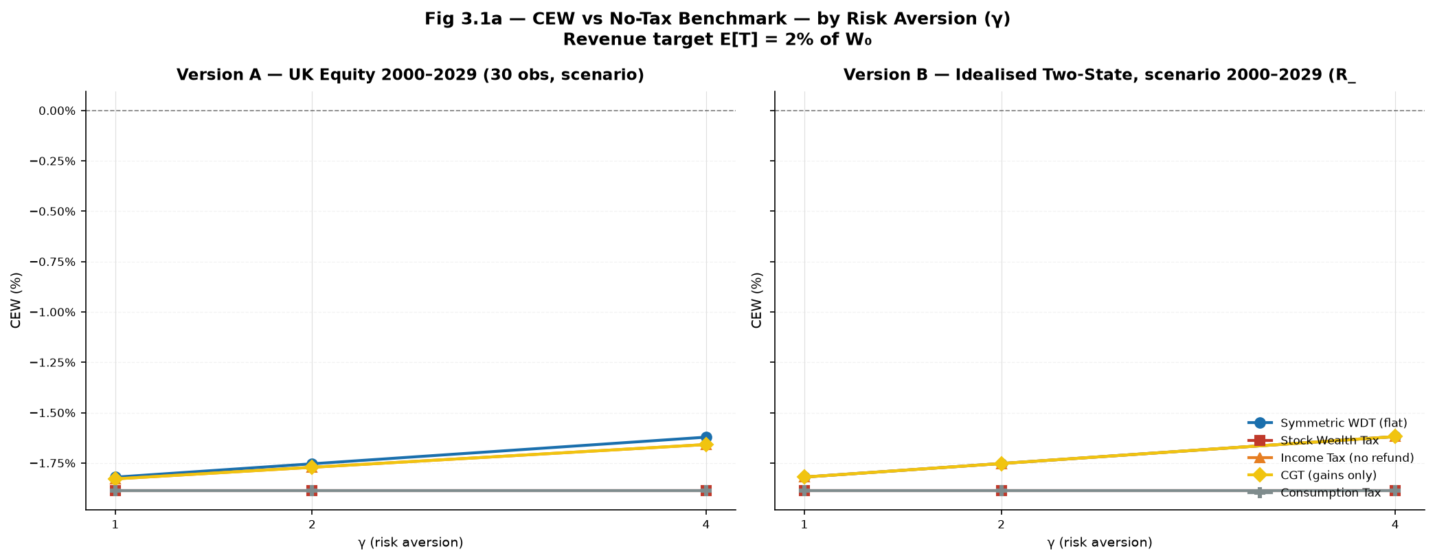
The flat WDT leads by 17.4 basis points over income tax and CGT, and by 133.1 basis points over stock wealth and consumption tax. Neither advantage is the paper’s primary conclusion. The baseline establishes fair ground — the WDT does not win through a mechanical rate advantage. Everything in Part II is attributable to mechanisms.
Two structural features of Table 1 recur throughout Part II.
The first is the exact clustering of stock wealth tax and consumption tax at −1.8870% across all values of γ and both distributions (WFR.A §A.1). Both systems apply a fixed proportional wedge to a base that does not condition on return performance. Under CRRA preferences, a fixed proportional wedge leaves the relative consumption distribution unchanged, making the risk-aversion parameter irrelevant. Welfare cost is determined entirely by revenue extracted, not by how extraction interacts with return risk. This γ-invariance is a structural property of these two bases, not a calibration coincidence. It also foreshadows the concentration result in (WFR §4.3): a tax base that does not condition on return performance does not attenuate the compounding of return differences across taxpayers.
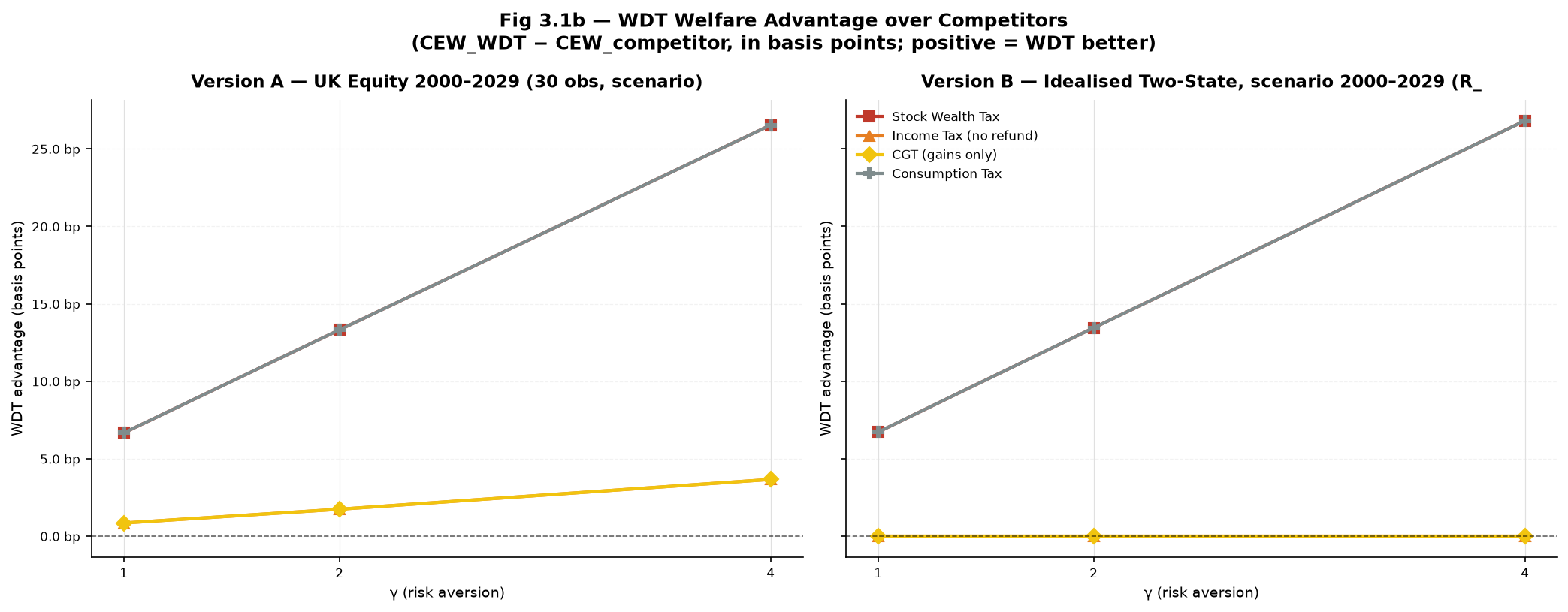
The second is the exact equality of income tax and CGT at −1.7713%. In a single-period model where all gains are realised each period, CGT is structurally identical to a gains-only income tax. The realisation decision is suppressed here. When it is admitted in (WFR §4.2), the welfare difference between the two systems becomes the largest in the paper. The baseline equality is the controlled condition that makes the lock-in cost in (WFR §4.2) attributable to the realisation mechanism alone.
Progressive WDT sits between the two clusters at −1.8288%, 74.9 basis points worse than flat WDT and 58.2 basis points better than the stock-base systems. This intermediate position reflects the logistic: at the canonical wealth levels tested, the logistic is operating near its entry rate \(\tau_0\) rather than its ceiling \(\tau_m\), so the progressive schedule diverges only modestly from the flat rate. The three complications this introduces to the Domar-Musgrave result are the subject of (WFR §4.1).
If structural welfare differences are small when distortions are suppressed, where does the actual welfare cost of existing systems come from? Part II answers this for each system in turn. The answer, in each case, is a mechanism that the delta base either eliminates by construction or substantially attenuates.
3.2 The D-M Risk-Sharing Property: Mechanism Established, Verdict Deferred
Domar & Musgrave (1944) establish that a proportional tax with full symmetric loss offsets leaves the agent’s optimal risky portfolio share unchanged. When the government taxes gains at rate \(\tau\) and refunds losses at the same rate, it participates proportionally in both the upside and the downside of every risky position. The gross return distribution is contracted by the factor (1−\(\tau\)) in every state. The relative ranking of return states is unchanged, the indifference condition for portfolio allocation is unchanged, and therefore the optimal portfolio is unchanged.
The flat symmetric WDT is a direct application of this mechanism to a wealth-delta base. The model confirms it holds to floating-point precision. Table 2 reports the Domar-Musgrave test across risk-aversion parameters and both distributions.
Table 2: Domar-Musgrave Test — Flat Symmetric WDT
| Distribution | γ | \(\tau\) | (1−\(\tau\))² | Actual ratio | Gap |
|---|---|---|---|---|---|
| Ver. A | 1 | 33.404% | 0.443505 | 0.443505 | −5.55×10⁻¹⁷ |
| Ver. A | 2 | 33.404% | 0.443505 | 0.443505 | −5.55×10⁻¹⁷ |
| Ver. A | 4 | 33.404% | 0.443505 | 0.443505 | −5.55×10⁻¹⁷ |
| Ver. B | 1 | 33.404% | 0.443505 | 0.443505 | 9.44×10⁻¹⁶ |
| Ver. B | 2 | 33.404% | 0.443505 | 0.443505 | 9.44×10⁻¹⁶ |
| Ver. B | 4 | 33.404% | 0.443505 | 0.443505 | 9.44×10⁻¹⁶ |
Ratio = Var(C_tax) / Var(C_notax). D-M predicts this equals (1−\(\tau\))². Gap = actual ratio minus predicted. Gaps are at floating-point precision (10⁻¹⁶ to 10⁻¹⁷). Full specification in (WFR.A §A.4).
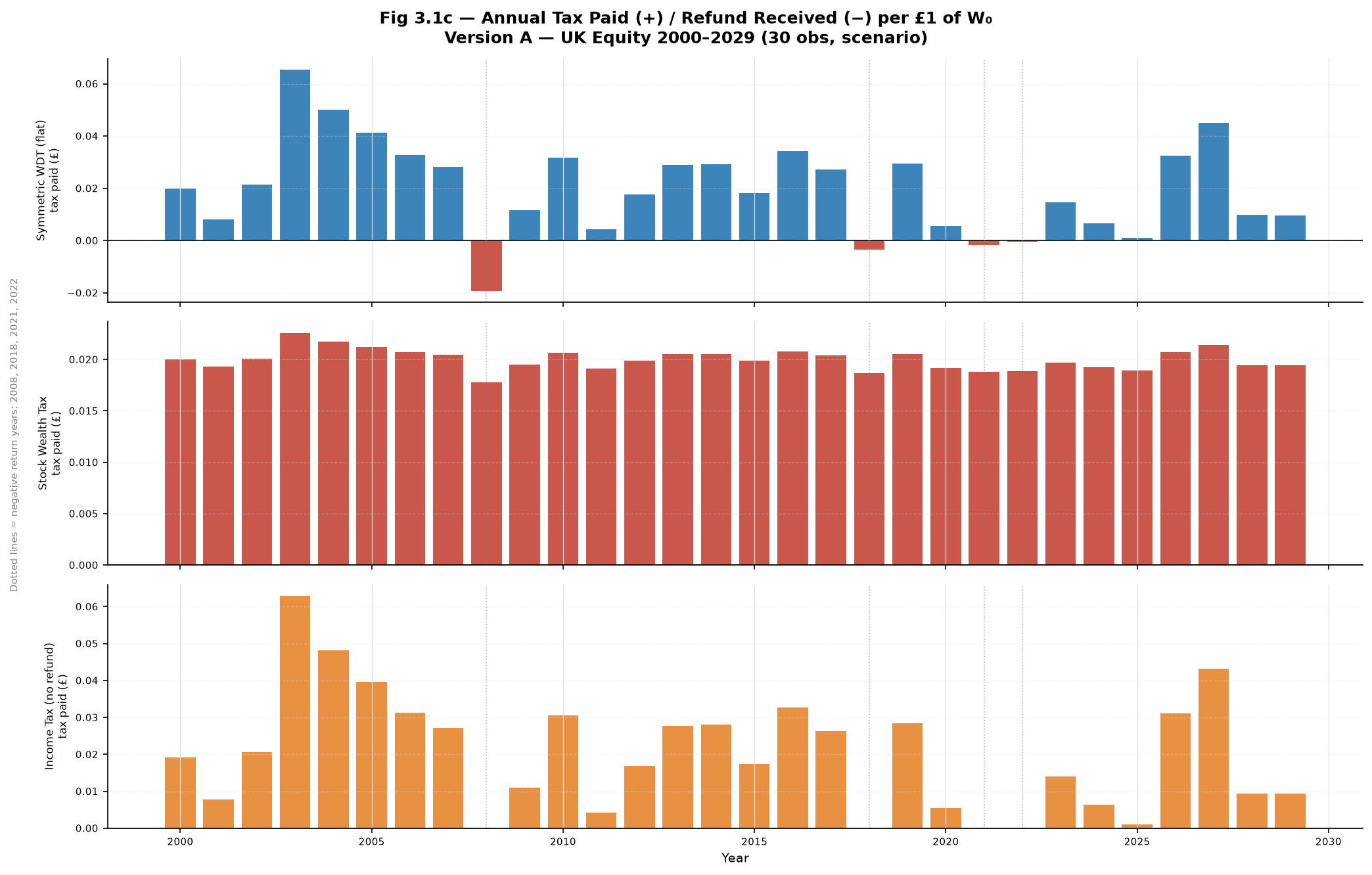
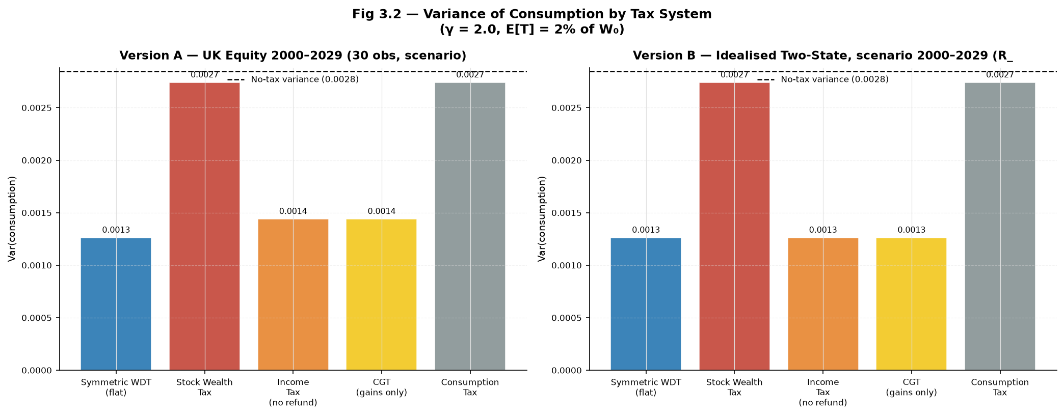
The consumption variance result in (WFR.A §A.2) confirms the mechanism from a different angle. At γ=2, the flat WDT produces Var(C) = 0.0013 — identical across both distributions. Income tax and CGT produce Var(C) = 0.0014 under Ver. A, approximately 8% higher. Stock wealth and consumption tax produce Var(C) = 0.0027, more than double the WDT figure. Among the systems modelled here, the WDT contracts the consumption distribution most tightly at revenue equivalence without distorting the relative ranking of return states.
D-M is a risk-sharing result, not a welfare-superiority result. It identifies the channel through which the flat symmetric WDT contracts consumption variance without creating the conventional risk-taking distortion. Whether the variance reduction translates into a welfare advantage depends on what distortions the competing systems impose and whether the WDT introduces distortions of its own. The welfare translation is the subject of Part II; the mechanism is established here.
This sequencing is not merely organisational. Arachi & D’Antoni (2022) establish that accrual taxation is not automatically welfare superior to realisation taxation, because accrual taxes bill unrealised gains before the taxpayer has liquidity to pay without adjusting consumption. Engaging with that objection requires first establishing what the WDT’s risk-sharing mechanism is before showing how the symmetric refund answers it. If the D-M result were presented as a welfare argument rather than a mechanism, the paper would appear to make exactly the claim Arachi et al. rebut. Section 4.2 shows why the WDT is not subject to that rebuttal, but that argument requires the mechanism established here as its foundation.
4. Part II: The Mechanisms
4.1 Progressive Rates: Three Complications, All Second-Order
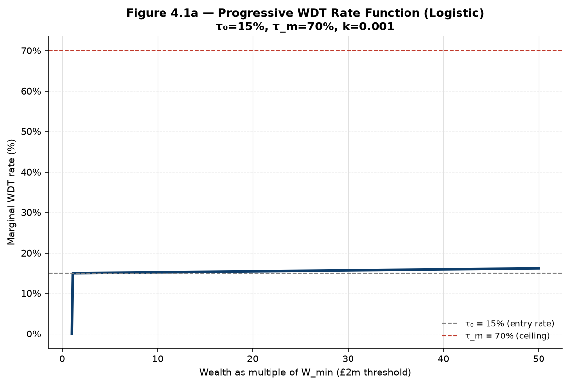
A progressive rate schedule breaks the Domar-Musgrave result from (WFR §3.2). The D-M derivation requires a flat proportional rate: the government’s co-investment share must be constant across all wealth levels for the contracted return distribution to leave risk rankings unchanged. Under a logistic progressive schedule, the effective rate varies with wealth, so the co-investment share varies too — gains in higher-wealth states are taxed more heavily than equivalent losses at lower post-loss wealth. This introduces three distinct complications to the D-M architecture. All three are real. All three are second-order at canonical parameters across the tested population.
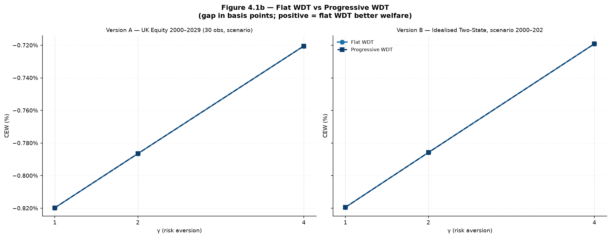
C1: Progression itself. The welfare gap between flat and progressive WDT — measured as (CEW_flat − CEW_progressive) × 10,000 — is the quantification of this effect in isolation. At the canonical test wealth of \(W_0\) = £10m (five times the entry threshold), the gap is −0.00 basis points across all γ and both distributions (WFR.A §B.1). The sweep across \(\tau_0\), \(\tau_m\), \(k\),and \(W_{min}\) in (WFR §4.5.3); full tables in (WFR.A §E.3.1) to (WFR.A §E.3.4) confirms the gap remains below 0.05 basis points even at \(W_0\) = £100m under all canonical parameter combinations. The logistic is operating on the near-flat lower limb at \(W_0\) = £10m with \(W_{min}\) = £2m and \(k\) = 0.001, where effective rates barely differ from \(\tau_0\). C1 would widen at wealth levels far above the inflection point, but across the population this model tests, it is empirically negligible.
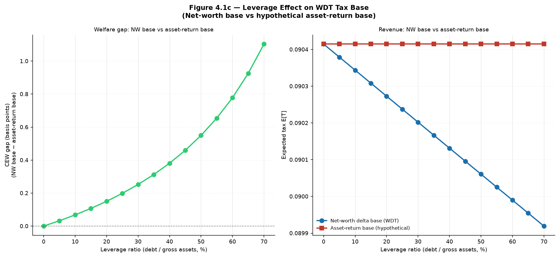
C2: The leverage and net-worth base interaction. The WDT applies to net worth W = A − D. An agent with leverage ratio D/A holds less net worth for a given gross asset position, so the WDT’s absolute tax burden is smaller than it would be on the underlying asset return alone. Table 3 reports the welfare gap between the WDT’s actual net-worth base and a hypothetical asset-return base across leverage ratios from 0% to 70%.
Table 3: Leverage Effect on WDT Tax Base and Welfare (Selected Rows)
| Leverage (%) | \(W_0\) net (£m) | CEW: NW base | CEW: asset-return base | Gap (bp) |
|---|---|---|---|---|
| 0.0 | £10.00m | −0.7865% | −0.7865% | +0.00 |
| 20.0 | £8.00m | −0.9501% | −0.9516% | +0.15 |
| 40.0 | £6.00m | −1.1995% | −1.2033% | +0.38 |
| 60.0 | £4.00m | −1.6228% | −1.6306% | +0.78 |
| 70.0 | £3.00m | −1.9602% | −1.9712% | +1.10 |
Full table in (WFR.A §B.2). Progressive rate function. γ=2. Ver. A distribution. Gross assets = £10m throughout.
The gap is monotone in leverage, rising from zero at no debt to +1.10 basis points at 70% leverage. The direction is unambiguous: as debt rises, net worth falls, reducing the absolute tax liability relative to the asset-return comparator. This is a real complication relevant to a policymaker deciding whether to apply the WDT to gross or net positions. At 1.10 basis points even at extreme leverage, it is second-order relative to the mechanisms in (WFR §4.2) to (WFR §4.3).
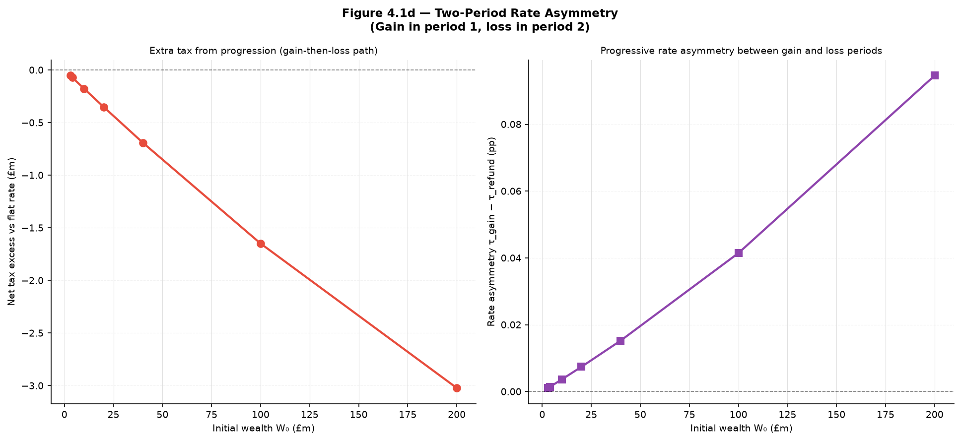
C3: Intertemporal rate asymmetry. Under a progressive schedule, a gain in period 1 increases wealth and attracts a higher effective rate than the refund received in period 2 on an equivalent loss, because the loss is assessed at the lower post-gain wealth level. This asymmetry is a property of any progressive tax with non-linear rates and gain-loss sequences. Table 4 reports the gain-refund rate differential and the net tax difference relative to the flat WDT benchmark across initial wealth levels.
Table 4: Two-Period Rate Asymmetry by Initial Wealth
| \(W_0\) (£m) | \(\tau\) gain (%) | \(\tau\) refund (%) | Asymmetry (pp) | Excess vs flat (£m) |
|---|---|---|---|---|
| 3.0 | 15.015 | 15.014 | +0.0011 | −0.0532 |
| 10.0 | 15.106 | 15.102 | +0.0037 | −0.1765 |
| 40.0 | 15.498 | 15.483 | +0.0153 | −0.6908 |
| 100.0 | 16.305 | 16.263 | +0.0415 | −1.6488 |
| 200.0 | 17.713 | 17.619 | +0.0946 | −3.0220 |
Full table in (WFR.A §B.3). Sequence: +18.8% gain period 1, −8.3% loss period 2. Excess = net tax progressive − net tax flat; negative means progressive WDT collects less than flat.
The asymmetry grows with wealth, from +0.0011 percentage points at £3m to +0.0946 percentage points at £200m, remaining small relative to the canonical \(\tau_0\) of 15%. The Excess column requires explanation because its sign is counterintuitive: progression collects less net tax than flat across the full wealth range tested. This is not a model error. The wealth levels tested sit in the near-flat region of the logistic, where effective rates are at or just above \(\tau_0\), well below the flat revenue-equivalent rate of 33.4%. The gain-at-higher-rate asymmetry that textbook treatment of progressive brackets would predict requires wealth to sit at or above the logistic inflection point, which the canonical population does not reach. C3 is a real and measurable complication; its direction in the current calibration is not the direction a reader familiar with progressive bracket asymmetry would expect.
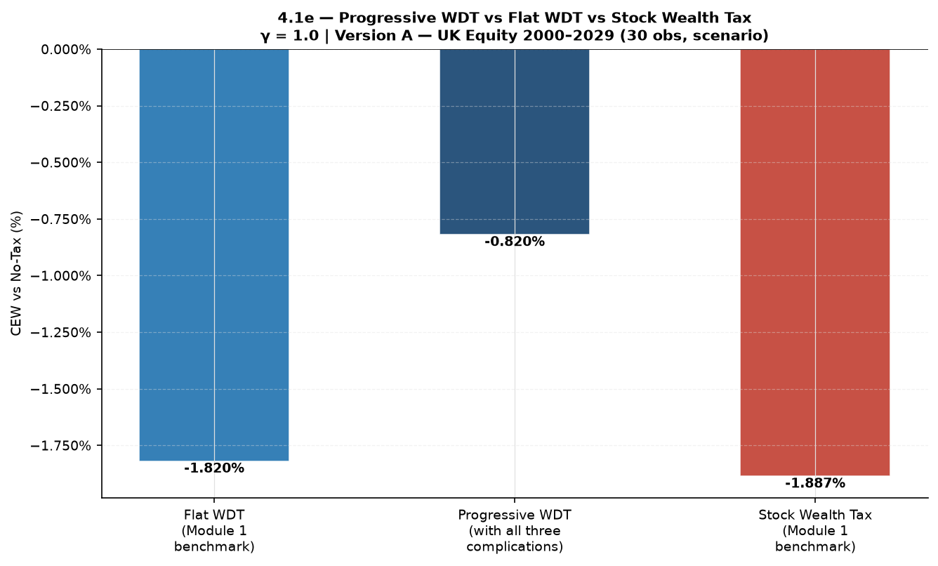
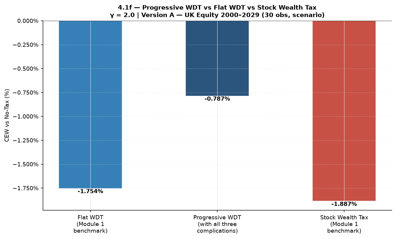
All three complications are real features of the logistic progressive schedule. None is large enough to alter the comparative welfare picture.

4.2 CGT Lock-In: The Dominant Welfare Result
4.2.1 The Endogenous Realisation Decision
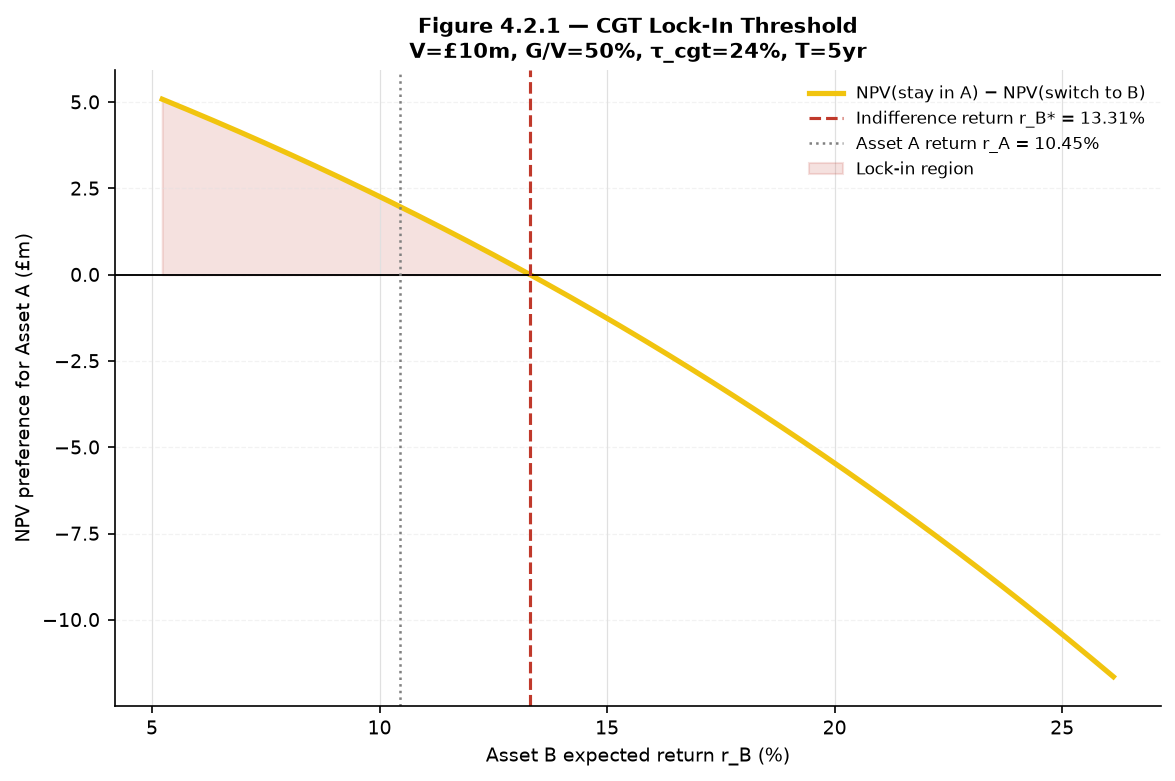
The baseline showed income tax and CGT at identical welfare levels — because the realisation decision was suppressed. In practice, a CGT taxpayer who holds asset A and observes that asset B offers a higher expected return faces a decision the baseline did not model: switching from A to B triggers a CGT liability on the embedded gain, creating a wedge between the gross return advantage of switching (r_B − r_A) and the net return from switching after tax. If the gain-to-value ratio G/V is large enough, or the remaining holding period T is short enough, the tax cost of switching exceeds the benefit of the superior return, and the rational response is to remain in the inferior asset.
This is lock-in — the rational response to the tax schedule, not a decision error. The wedge is larger when embedded gains are larger relative to asset value, when the remaining investment horizon is shorter, and when the CGT rate is higher.
The indifference return r_B* is the minimum return on asset B at which the agent will switch given the CGT liability on the existing position: the NPV of remaining in A equals the NPV of switching to B and paying the CGT on exit. At the reference calibration (G/V = 50%, T = 5, \(\tau_{cgt}\) = 24%, r_A = 10.45%), r_B* = 13.31% — almost three percentage points above r_A. Any asset B offering a return between 10.45% and 13.31% would be preferred to asset A without CGT but is not worth the switching cost given the embedded liability.
4.2.2 The Welfare Cost of Lock-In
Table 5 reports the full welfare comparison between the WDT and CGT once the realisation decision is endogenous.
Table 5: WDT vs CGT — With and Without Lock-In
| Metric | Ver. A (Empirical) | Ver. B (Idealised) |
|---|---|---|
| Flat WDT CEW | −1.7539% | −1.7525% |
| CGT CEW (no lock-in) | −1.7713% | −1.7525% |
| Lock-in welfare cost | +141.22 bp | +41.19 bp |
| CGT CEW (with lock-in) | −3.1834% | −2.1644% |
| WDT advantage (no lock-in) | +1.74 bp | +0.00 bp |
| WDT advantage (with lock-in) | +142.96 bp | +41.19 bp |
| P(agent locked in) | 90.0% | 100.0% |
| CGT indifference return r_B* | 13.31% | 13.31% |
Reference calibration: G/V = 50%, T = 5 years, \(\tau_{cgt}\) = 24%, r_A = 10.45%, γ = 2. Full table in (WFR.A §C.3).
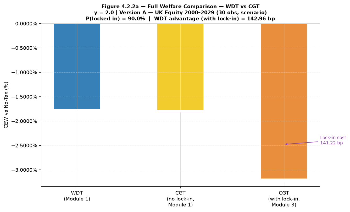
The WDT advantage grows from 1.74 basis points without lock-in to 142.96 basis points with lock-in — approximately 82 times the baseline difference. The mechanism is not a rate advantage: the revenue-equivalent CGT rate is 32.07% versus the WDT’s 33.40%. CGT is cheaper at revenue equivalence. The welfare cost arises entirely from the lock-in distortion — the portfolio misallocation the realisation contingency enforces.
Ver. A and Ver. B results diverge considerably: 142.96 versus 41.19 basis points. The empirical distribution includes negative return years in which CGT collects nothing but the WDT provides refunds. These years require a lower revenue-equivalent CGT rate (32.07% versus 33.40%), which reduces the switching wedge slightly — but more importantly, the empirical distribution’s fat left tail generates more states in which the agent is locked into a loss-making position without tax relief. The idealised Ver. B distribution smooths over these states, understating both the lock-in cost and the WDT’s revenue-equivalence rate advantage.
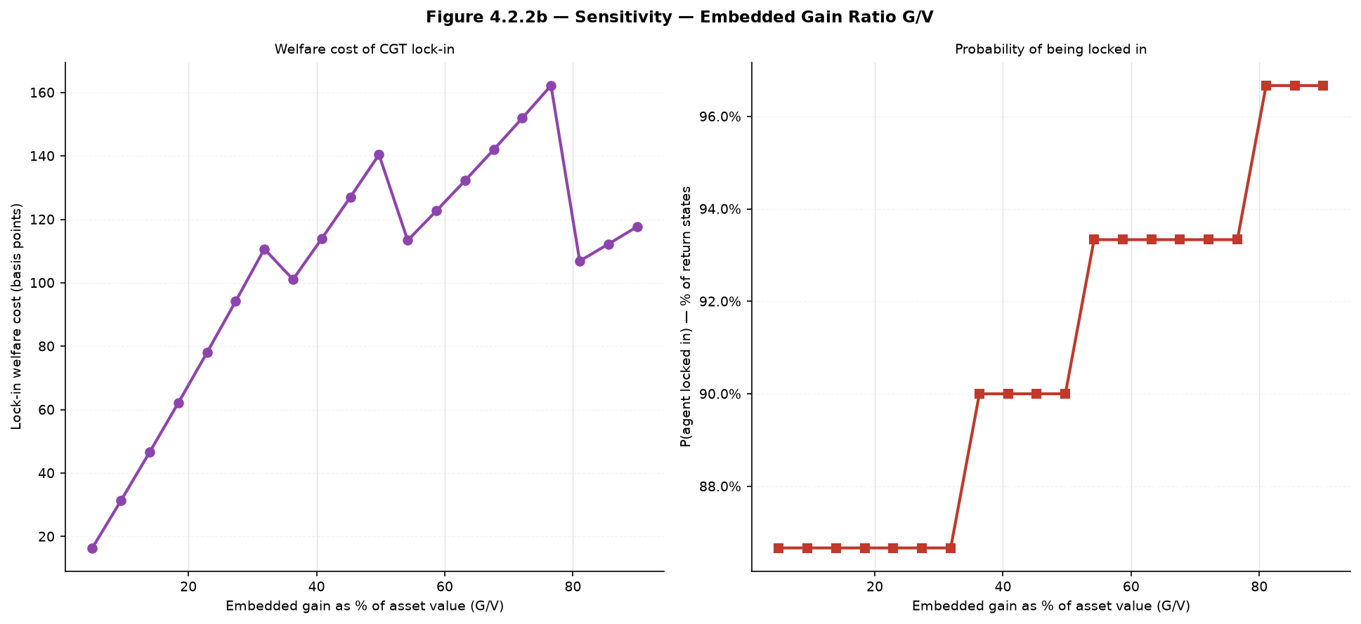
The G/V sweep. The lock-in cost varies substantially with the embedded gain ratio. Table 6 reports selected rows from the full sweep in (WFR.A §C.1).
Table 6: Lock-In Welfare Cost by Embedded Gain Ratio (Selected Rows)
| G/V (%) | Lock-in cost (bp) | P(total locked) | P(CGT distortion) | P(r_B < r_A) |
|---|---|---|---|---|
| 5.0 | +16.4 | 86.7% | 0.0% | 86.7% |
| 31.8 | +110.7 | 86.7% | 0.0% | 86.7% |
| 49.7 | +140.4 | 90.0% | 3.3% | 86.7% |
| 67.6 | +142.0 | 93.3% | 6.7% | 86.7% |
| 76.6 | +162.2 | 93.3% | 6.7% | 86.7% |
| 81.1 | +106.9 | 96.7% | 10.0% | 86.7% |
Full table in (WFR.A §C.1). Ver. A distribution, γ=2, T=5.
The lock-in cost rises from +16.4 basis points at G/V = 5% to a peak of +162.2 basis points at G/V = 76.6%, then falls non-monotonically above G/V = 81%. That non-monotonicity is a discretisation artefact: as r_B* rises with the embedded gain, it approaches the upper boundary of the empirical return distribution, and the probability of any return state exceeding r_B* shrinks rapidly. States generating lock-in costs are absorbed into the P(r_B < r_A) category as r_B* crosses above r_A for an increasing share of the distribution. This is a boundary effect of the finite empirical distribution, not a meaningful economic result.
The P-decomposition columns require precise reading and the distinction between them carries the welfare interpretation. P(remain in A) combines two structurally different situations: states where r_B < r_A — the agent stays because asset B is simply inferior to asset A, with or without CGT — and the CGT distortion proper, states where r_A ≤ r_B < r_B*, where the agent would switch to the superior asset without CGT but the switching cost makes it irrational to do so. At G/V = 5%, P(remain in A) is 86.7% with P(CGT-induced non-switching) = 0.0%: every non-switching state is market preference, not tax distortion. The CGT distortion proper only begins above G/V = 36.3%. At the reference calibration of G/V = 50%, P(CGT-induced non-switching) = 3.3% while P(r_B < r_A) = 86.7%. The welfare cost attributable to CGT is generated by that 3.3 percentage point distortion zone, not by the 86.7% of states where the agent would stay regardless of the tax regime. Conflating the two components would substantially overstate the CGT’s role in driving non-switching probability.
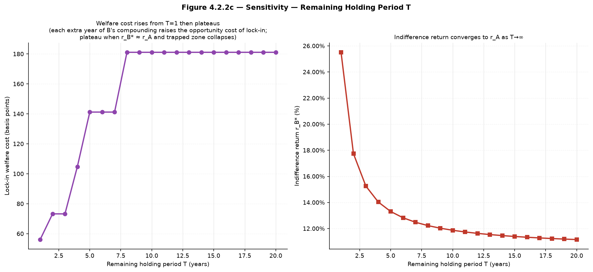
The T sweep. Table 7 reports the lock-in cost across holding periods at G/V = 50%.
Table 7: Lock-In Welfare Cost by Remaining Holding Period (Selected Rows)
| T (years) | r_B* (%) | Lock-in cost (bp) | P(CGT distortion) |
|---|---|---|---|
| 1 | 25.51% | +56.1 | 13.3% |
| 2 | 17.74% | +73.3 | 10.0% |
| 5 | 13.31% | +141.2 | 3.3% |
| 8 | 12.23% | +181.1 | 0.0% |
| 20 | 11.16% | +181.1 | 0.0% |
Full table in (WFR.A §C.2). G/V = 50%, Ver. A distribution, γ=2.
The welfare cost rises from +56.1 basis points at T = 1 to a plateau of +181.1 basis points from T = 8 onward. The direction is unambiguously upward. At T = 1, the agent has only one period to benefit from switching to asset B. Each additional year compounds the foregone return advantage of remaining misallocated.
The plateau from T = 8 requires careful interpretation. At that point, r_B* has converged close enough to r_A that no empirical return state falls in the wedge between them: P(CGT-induced non-switching) reaches 0.0%. Yet the welfare cost is at its maximum. This is not a contradiction. What the model is capturing from T = 8 onward is better described as realisation-induced portfolio persistence: the initial switching decision — made rational by the CGT liability at the outset — propagates across all subsequent periods as a compounding allocation error. The agent is not being prevented from switching in each of those years by an ongoing distortion; they are paying the cumulative consequence of the initial misallocation the CGT induced. The 181 bp figure is the CEW cost of that multi-period trajectory relative to the undistorted benchmark, not a measure of annual lock-in probability.
4.2.3 The Arachi Pivot
Arachi & D’Antoni (2022) establish that accrual taxation is not automatically welfare superior to realisation-based taxation. Their argument: an accrual tax bills unrealised gains before the taxpayer has received the cash to pay without altering consumption. In years when asset values have risen but no sale has occurred, the taxpayer must either draw down liquid reserves, adjust consumption downward, or borrow — all of which create intertemporal consumption distortions that realisation-based taxation avoids. This is the most technically serious theoretical counterargument to any accrual-based tax proposal.
The WDT is an accrual-based tax. The Arachi objection applies to accrual proposals that do not specifically address the mechanism through which accrual creates intertemporal distortions. Whether it applies to the WDT depends on what the symmetric refund does and does not do.
The symmetric refund directly addresses the loss-year component of the Arachi objection. In any year in which net worth falls, the WDT pays a refund proportional to the loss. The refund is delivered at exactly the moment when the taxpayer’s wealth has declined — when liquid reserves are most strained and when the Arachi distortion would otherwise be most acute. The government does not merely collect less in a bad year; it actively transfers purchasing power to the taxpayer when the taxpayer’s position has deteriorated.
This makes the WDT structurally different from every prior accrual tax proposal. All earlier accrual proposals — the Vickrey averaging system, the Bradford X-tax accrual variant, prior rate-of-return allowance designs — either did not include full symmetric loss refunds or imposed conditions limiting refund access in precisely the years when loss relief is most valuable.
The objection nonetheless applies at the entry margin. The lifetime contribution envelope caps cumulative refunds at cumulative taxes paid by each taxpayer to date (WP §3.5). A taxpayer who enters the WDT in a loss year — before any cumulative tax has been paid — cannot receive a refund, because the envelope floor binds at zero. This is the situation of the Poor tier in (WFR §4.3), where the envelope binds in the scenario’s first year. At that margin, the Arachi distortion applies in full: the taxpayer faces wealth deterioration without compensating transfer.
The envelope floor also limits the mechanism’s SRR exposure in this case: a taxpayer with zero cumulative contribution balance has zero refund entitlement, so the SRR faces no liability from early-year loss entrants. Whether a design extension providing an entry-year credit to new taxpayers experiencing early losses would be welfare-improving is a named trade-off under the MF §9 framework (it would reopen the exploitation surface CLOSE §8.4 identifies), left as a Governing Council calibration question rather than a current design requirement.
The symmetric refund therefore substantially changes the Arachi mechanism for established taxpayers with a positive cumulative contribution balance. At the entry margin where the envelope floor binds, the objection remains applicable. The WDT is not a general rebuttal of the Arachi critique; it is a design that relocates the distortion from the general case to the entry boundary.
4.2.4 Category Classification
The lock-in welfare cost — 141–143 basis points at the reference calibration under Ver. A — is a Category 1 finding: a welfare cost of an existing, operating system. It requires no WDT implementation data. A government that chose to maintain CGT after reviewing this analysis would be choosing to accept a welfare cost of this magnitude at plausible UK parameters, relative to any system that does not make the switching decision tax-relevant.
The magnitude is the model’s contribution at this calibration and is not claimed to be an externally validated general estimate of CGT lock-in costs. The mechanism is very strongly supported in the existing literature (WFR §5.3). What the model establishes is that across plausible UK parameter ranges, the lock-in cost is large — substantially larger than the baseline welfare differences across systems in Part I.
The WDT’s structural elimination of lock-in is a Category 2 property. The delta base does not make the switching decision between assets tax-relevant: switching from asset A to asset B changes the future return stream to which the delta base is applied, but does not trigger a realisation event and does not create a switching wedge. Lock-in cannot arise under the WDT by construction, not by calibration. Whether the WDT introduces its own intertemporal distortions — through the entry-margin envelope-binding case discussed in (WFR §4.2.3), implementation friction, valuation error under Route D, or compliance complexity — is a Category 3 question, named in (WFR §6.1.3) and not dismissed here.
4.3 Heterogeneous Returns: Concentration Under the Fagereng Premise
4.3.1 The Fagereng Premise and the Four-Tier Calibration
Fagereng et al. (2020), using Norwegian administrative data covering virtually the entire wealth distribution, establish three properties of individual investment returns directly relevant to tax-base design. First, there is substantial within-asset-class return heterogeneity: the gap between the 10th and 90th percentile of individual returns on broadly similar assets is approximately 18 percentage points. Second, returns are positively correlated with wealth level. Third, this heterogeneity is highly persistent: an individual’s return rank is a strong predictor of their return rank a decade later.
When returns differ persistently and are wealth-correlated, the choice of tax base determines whether the tax system attenuates or compounds the concentration process. A tax base conditioning on return performance collects more from high-return taxpayers in proportion to their gains; a stock base collects the same proportion regardless of how differently their wealth is growing.
The model uses a four-tier calibration drawn from Fagereng et al. (2020). Tiers are defined by their return differential relative to the UK historical equity mean of 10.45%: Poor (−4.55pp, approximate 95th wealth percentile), Ok (−2.05pp, 99th), Good (+0.95pp, 99.9th), and Great (+3.45pp, 99.99th+). Initial wealth levels are £2.9m, £7.1m, £19.9m, and £139.6m respectively. The 8pp gap between the outer tiers is conservative relative to Fagereng’s full 18pp distribution; the concentration results reported here are therefore a lower bound on the effect the Fagereng mechanism would produce at the full empirical return spread.
4.3.2 The Concentration Result
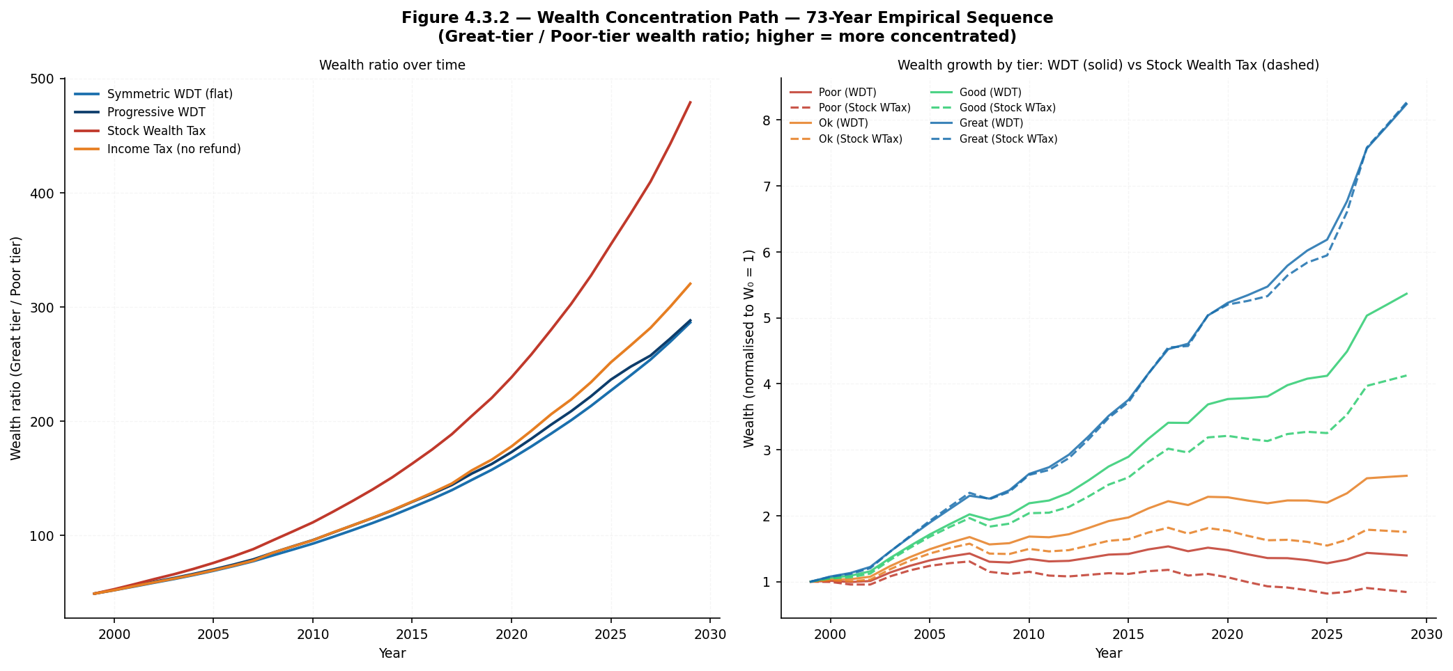
Table 8 reports the Great/Poor wealth ratio at five points across the 30-year scenario horizon starting in 2000.
Table 8: Wealth Concentration Path — Great/Poor Ratio at Key Years
| System | Initial | 2004 | 2009 | 2019 | 2029 (N=30) |
|---|---|---|---|---|---|
| Flat WDT | 48.8× | 65.1× | 87.4× | 157.2× | 286.3× |
| Progressive WDT | 48.8× | 66.1× | 90.3× | 162.3× | 288.1× |
| Income Tax | 48.8× | 65.5× | 90.2× | 166.1× | 320.2× |
| Stock Wealth Tax | 48.8× | 70.5× | 103.3× | 220.1× | 479.0× |
| Consumption Tax | 48.8× | 70.5× | 103.3× | 220.1× | 479.0× |
Initial ratio reflects \(W_0\) difference only. All systems calibrated at population-weighted aggregate revenue equivalence. Full series in (WFR.A §D.3).
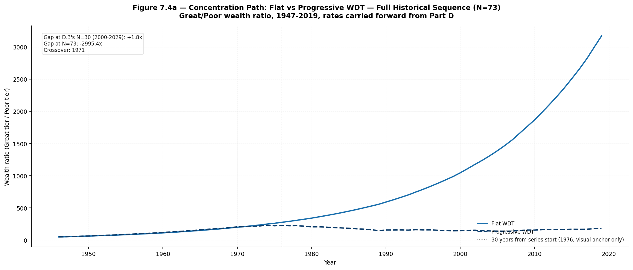
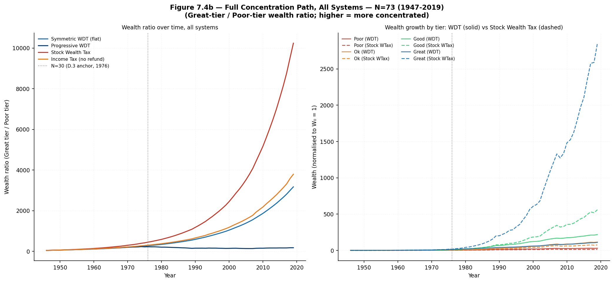
The dominant finding is the two-way split at N=30: the relevant axis is accrual basis versus stock base, not flat versus progressive rate. Both WDT variants reach approximately 286–288×; income tax reaches 320×; both stock-base systems reach 479×. The gap between the WDT variants at N=30 is 1.8× — smaller than the gap between either WDT variant and income tax (33–34×), which is itself smaller than the gap between income tax and the stock-base systems (159×).
This is an honest finding and should be stated as such. The progressive rate schedule does not produce meaningfully lower concentration than the flat rate at the canonical 30-year horizon. The Fagereng return differential of +8pp dominates the progressive versus flat rate differential at canonical logistic parameters over this horizon: the logistic has not risen far enough above \(\tau_0\) to compound a material difference in effective rate burden between tiers. A longer horizon would eventually reveal the progressive advantage, but it is outside the 30-year canonical window. The paper acknowledges this scope limitation rather than suppressing it.
The mechanism driving the 479× outcome for stock-base systems is structural. A stock wealth tax and a consumption tax both levy proportionally on wealth regardless of return. The Great-tier taxpayer earning 3.45pp above the mean and the Poor-tier taxpayer earning 4.55pp below it pay the same proportional charge on the same stock of wealth each period. The gap compounds at the full Fagereng rate across all 30 years, producing 479×. The delta base changes this by construction: a poor-return year generates a lower WDT charge or a refund, reducing the net wealth drain on the low-return taxpayer relative to the high-return taxpayer. The compounding differential is attenuated, not eliminated — hence WDT reaches 286× rather than holding concentration constant.
4.3.3 Within-Tier Welfare
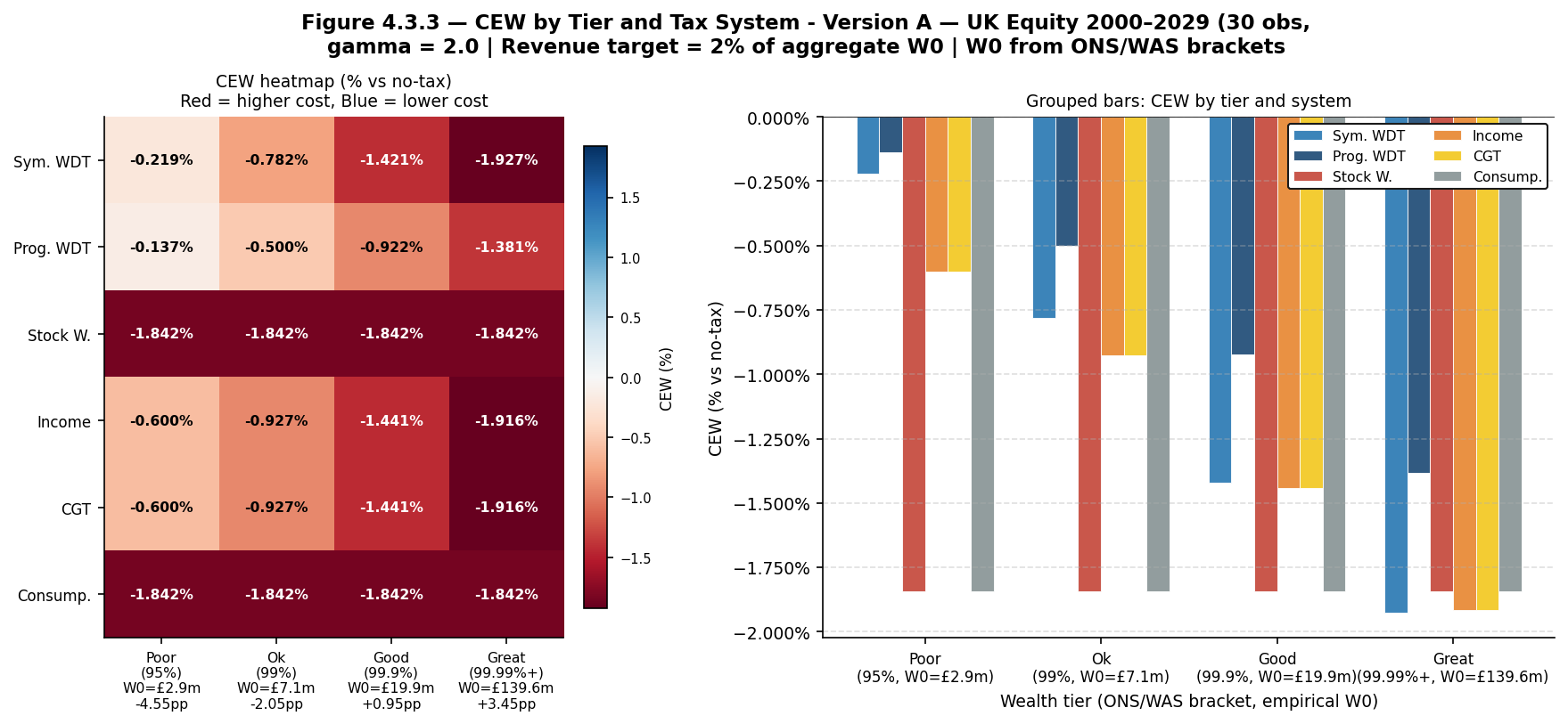
Table 9 reports CEW by tier and system.
Table 9: Certainty-Equivalent Welfare by Tier and Tax System
| System | Poor | Ok | Good | Great |
|---|---|---|---|---|
| Progressive WDT | −0.1375% | −0.5004% | −0.9223% | −1.3814% |
| Flat WDT | −0.2194% | −0.7816% | −1.4211% | −1.9269% |
| Income Tax | −0.6000% | −0.9274% | −1.4413% | −1.9161% |
| CGT | −0.6000% | −0.9274% | −1.4413% | −1.9161% |
| Stock Wealth Tax | −1.8424% | −1.8424% | −1.8424% | −1.8424% |
| Consumption Tax | −1.8424% | −1.8424% | −1.8424% | −1.8424% |
Tier wealth levels: Poor £2.9m, Ok £7.1m, Good £19.9m, Great £139.6m. γ=2, Ver. A. Full table in (WFR.A §D.1).
The sharpest within-tier result is at the Poor tier. Flat WDT delivers −0.2194% versus income tax’s −0.6000% — a gap of 38.1 basis points in the Poor tier’s favour. Progressive WDT widens this to 46.3 basis points. The mechanism is the symmetric refund: the Poor tier’s −4.55pp return differential means this tier spends more scenario years in negative-return states than any other. In those years, the WDT pays a refund; income tax collects nothing and provides nothing. Income tax’s structural asymmetry — participating in gains through collection but not in losses through relief — falls hardest on the taxpayer most frequently in loss states.
Progressive WDT provides better welfare than flat WDT at every tier. At the Poor tier, the improvement is 8.2 basis points; at the Great tier it is 54.6 basis points — the redistribution mechanism is working as designed, with higher logistic rates at the Great tier transferring burden upward. Stock wealth and consumption tax are welfare-equivalent across all tiers at −1.8424%, reflecting the γ-invariance result from (WFR §3.1) operating uniformly across the wealth distribution.
4.3.4 Distributional Incidence
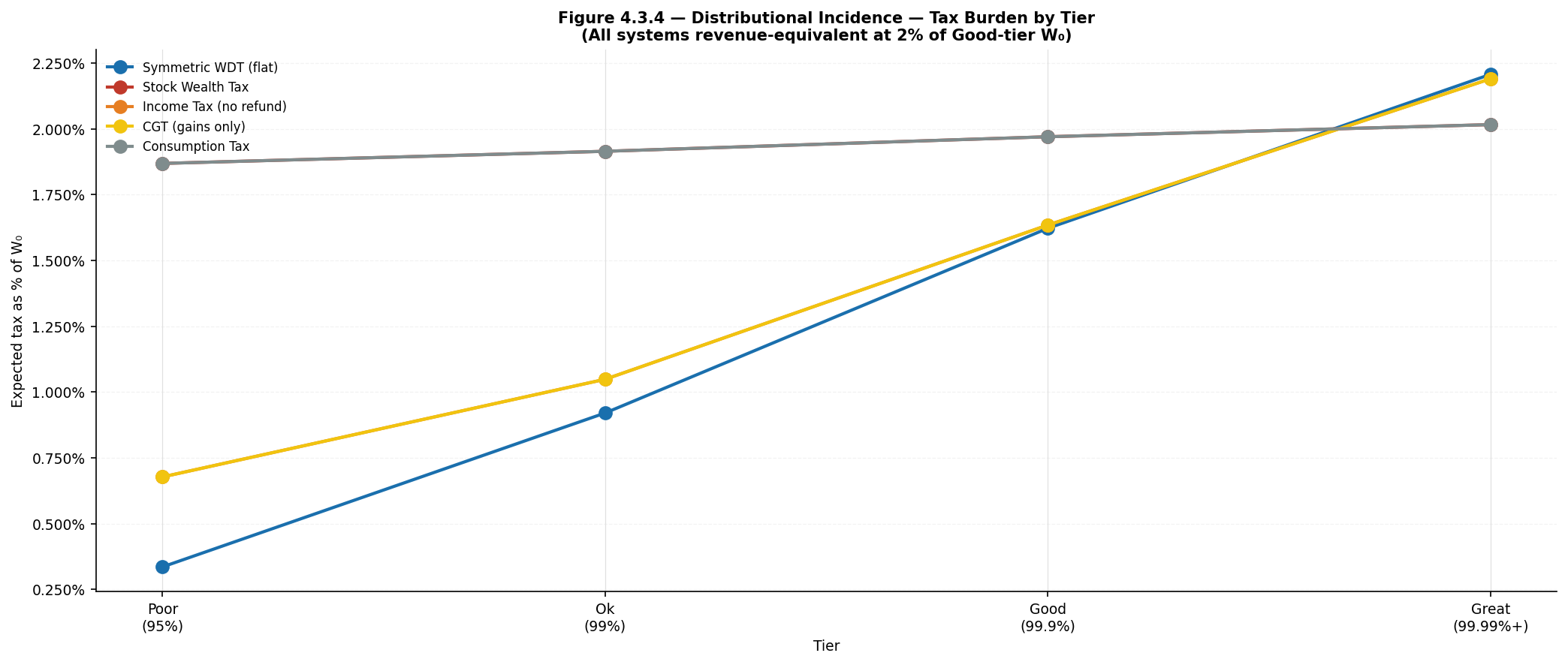
Table 10 reports expected tax as a percentage of \(W_0\) by tier.
Table 10: Distributional Incidence — Expected Tax as % of \(W_0\)
| System | Poor | Ok | Good | Great | Great/Poor ratio |
|---|---|---|---|---|---|
| Flat WDT | 0.34% | 0.92% | 1.62% | 2.21% | 6.6:1 |
| Income Tax | 0.68% | 1.05% | 1.63% | 2.19% | 3.2:1 |
| CGT | 0.68% | 1.05% | 1.63% | 2.19% | 3.2:1 |
| Stock Wealth Tax | 1.87% | 1.92% | 1.97% | 2.02% | 1.1:1 |
| Consumption Tax | 1.87% | 1.92% | 1.97% | 2.02% | 1.1:1 |
E[T]/\(W_0\) × 100. Full table in (WFR.A §D.2).
The WDT’s Great/Poor incidence ratio of 6.6:1 substantially exceeds income tax’s 3.2:1, despite both systems being calibrated to the same aggregate revenue target. The WDT’s delta base scales with both wealth and the return differential, because the tax applies to net-return × \(W_0\). The Great tier earns 3.45pp above the mean on £139.6m; the Poor tier earns 4.55pp below the mean on £2.9m. The product of wealth and outperformance is highly concentrated at the Great tier, so the delta base collects disproportionately from the highest-return taxpayers. Income tax also collects more from high-return taxpayers, but applies to gross gains rather than net returns above a cost-of-capital allowance, so the scaling is less pronounced. Stock and consumption tax incidence is near-flat at 1.1:1 — the stock base collects proportionally to wealth regardless of returns.
The aggregate revenue equivalence produces these tier-level differences by construction: the comparison is calibrated so that the same total revenue is raised across the population, not so that each tier pays the same rate. A referee who observes that the WDT’s Poor-tier burden is 0.34% against income tax’s 0.68% should read this as a consequence of the accrual base: a taxpayer earning 4.55pp below the mean on a modest wealth base generates a small positive or negative delta each year, and the WDT accordingly collects little from them.
These two dimensions — tax incidence and welfare incidence — should be read separately, not conflated. The WDT’s 6.6:1 Great/Poor incidence ratio is a more progressive tax burden than income tax’s 3.2:1. Its Poor-tier CEW of −0.2194% versus income tax’s −0.6000% is a more favourable welfare outcome for the same tier. Both results run in the same direction, but they measure different things. A higher incidence ratio means the high-return tier pays more relative to the low-return tier. A lower CEW cost at the Poor tier means the low-return tier is better off under this system on the model’s welfare criterion. Whether more progressive tax incidence is inherently preferable to less progressive incidence depends on a social welfare function this paper does not specify. The CEW comparison — which is within the paper’s stated welfare criterion — is the defensible claim; the incidence ratio is a distributional property, valuable as a description but not, on its own, a welfare result.
4.3.5 The Lifetime Contribution Envelope — Binding Result
Table 11 reports the envelope binding status across tiers under flat WDT over the 30-year scenario.
Table 11: Lifetime Contribution Envelope — Binding Summary
| Tier | \(W_0\) (£m) | Cumulative tax | Cumulative refund | Min slack | Ever binds? |
|---|---|---|---|---|---|
| Poor | £2.9m | £0.473m | £0.270m | £0.000m | ⚠ Yes (2001) |
| Ok | £7.1m | £2.440m | £0.398m | £0.042m | No |
| Good | £19.9m | £16.503m | £0.310m | £0.210m | No |
| Great | £139.6m | £330.303m | £1.423m | £2.210m | No |
Min slack = minimum of (cumulative tax − cumulative refund) over the 30-year window. Zero = envelope exactly reached. Full table in (WFR.A §D.4).
The Poor tier’s envelope binds in 2001 — the first assessment year of the scenario. The Poor tier’s −4.55pp return differential produces a loss in the opening year before any cumulative tax has been paid, so the refund is capped at zero. For all other tiers the envelope does not bind across the 30-year window.
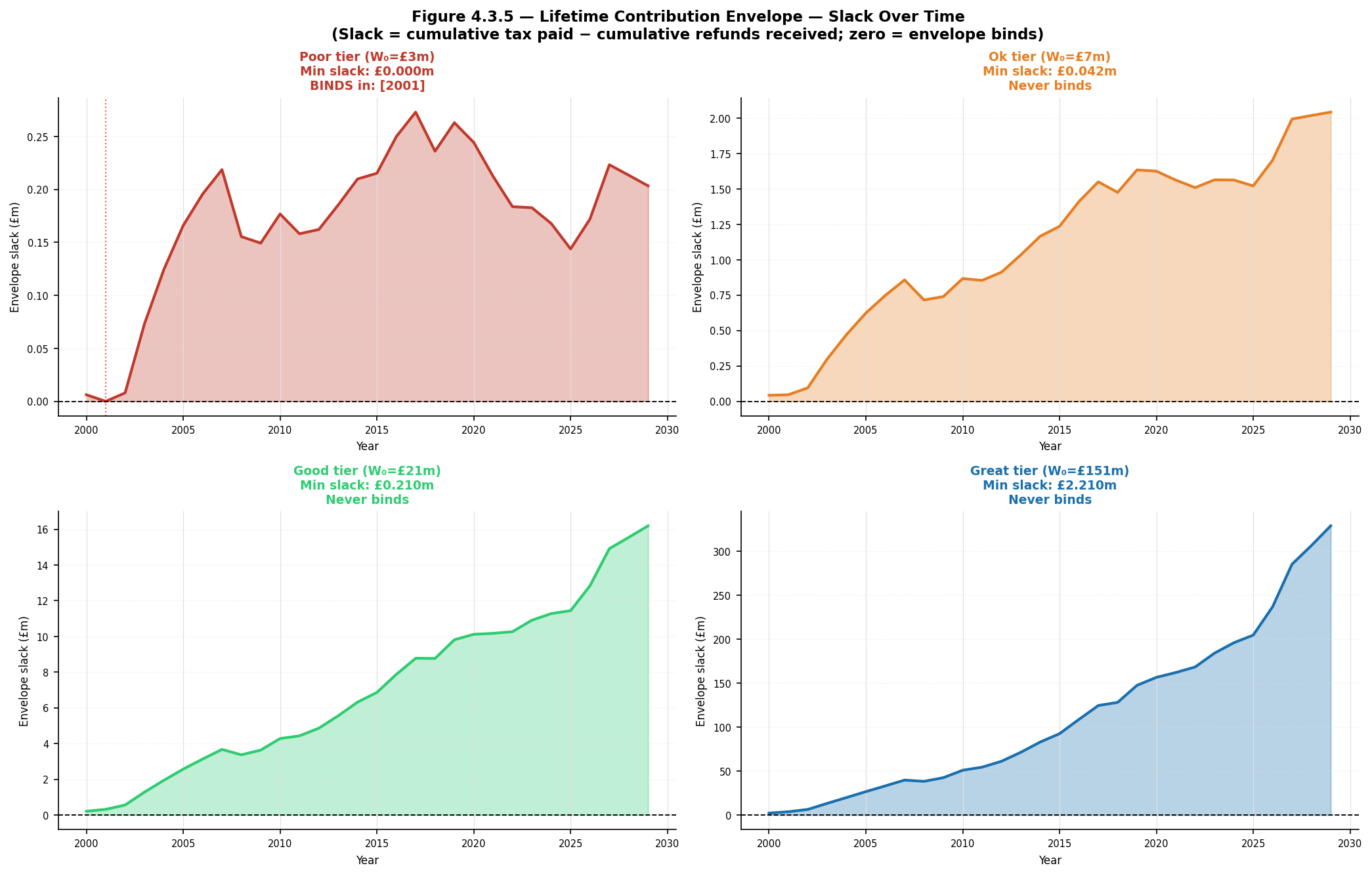
The lifetime contribution envelope bounds taxpayer-level lifetime refund exposure: refund obligations can never exceed cumulative receipts from any taxpayer whose envelope is not binding. This eliminates the risk of open-ended actuarial exposure at the individual taxpayer level. It does not eliminate aggregate liquidity risk at the SRR level: for taxpayers who enter the system in a loss year with no prior contribution history, the government must either pre-fund the SRR from non-WDT sources or provide an initial credit against future taxes. That is a liquidity timing requirement for the SRR, not a structural funding shortfall — the Poor-tier taxpayer who receives no refund in 2001 will generate positive contributions in subsequent gain years — but it is a real initial-cohort capitalisation requirement, not a risk that is absent by construction. The result here holds for the 2000-start scenario; the full start-year distribution is in (WFR §4.5.2); tables in (WFR.A §E.2).
As noted in (WFR §4.2.3), this is also the boundary condition under which the Arachi objection applies in full: the Poor-tier entrant in a loss year does not receive the symmetric refund that makes the WDT’s accrual structure welfare-superior to realisation-based taxation. This is a scope limitation of the design at the entry margin, not a failure of the mechanism in the general case.
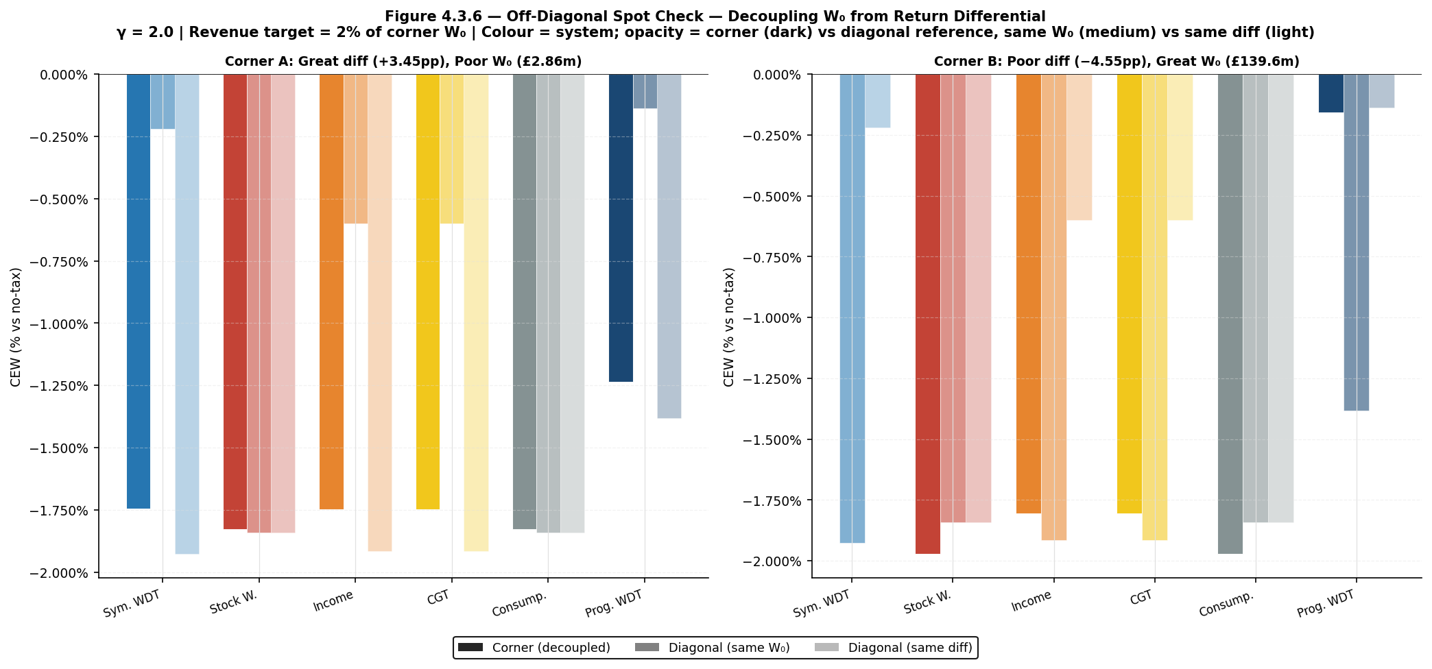
4.3.6 The Off-Diagonal Cell
Table D.5 reports a spot check that decouples initial wealth from return differential — examining what happens when a Poor-level return differential is applied to Great-level wealth, and vice versa. The “—” entry for Corner B Symmetric WDT is explained in full in (WFR.A §D.5): the parameter combination lies outside the feasible calibration space for a flat symmetric refund at Great-tier wealth with a persistently negative return differential, and the revenue-equivalence solver does not converge.
4.4 Stock Wealth and Consumption Taxes: Equivalence and Concentration
The controlled baseline showed stock wealth tax and consumption tax clustered at exactly −1.8870% CEW. Table 8 showed them reaching the same 479× concentration at N=30. Both results have the same explanation.
The welfare equivalence. Both systems apply a fixed proportional wedge to a base that does not condition on return performance. The stock wealth tax applies a rate to the end-of-period stock of wealth; the consumption tax applies a rate to the flow of consumption, which in this model equals wealth growth net of the tax. In a single-period model with no labour income, no heterogeneous saving, and no liquidity constraints, both bases produce the same proportional compression of the consumption distribution across all return states. CRRA scale-invariance then makes the risk-aversion parameter irrelevant: welfare cost is determined entirely by revenue extracted, not by how extraction interacts with return risk.
This equivalence is a model-structural property under specific simplifying assumptions. It breaks as soon as the model is relaxed. Labour income changes the consumption-expenditure identity. Heterogeneous saving rates mean the two bases fall on different totals for the same taxpayer. Liquidity constraints create a wedge between the two systems in years when the consumption tax would require drawing down non-liquid wealth. Life-cycle structure introduces age-specific consumption patterns that interact differently with the two bases.
The concentration equivalence and its mechanism. The 479× result for both systems at N=30 is a Category 1 finding. Both stock-base systems reach this ratio because neither conditions on the difference between the taxpayer’s return and any cost-of-capital benchmark. The full 8pp return differential compounds unattenuated across all 30 years, producing 479× from an initial 48.8×. The delta base eliminates this by construction: it taxes the return in excess of the benchmark, not the stock. A Poor-tier loss year generates a refund; a Great-tier gain year generates a large positive tax. The differential compounds more slowly because the tax system participates asymmetrically in proportion to the return differential rather than treating both taxpayers identically on the stock they hold.
The 479× versus 286–288× contrast is the concentration mechanism stated in numbers. It is a Category 1 finding for the stock-base systems and a Category 2 property of the delta base: the attenuation follows from the structure of the tax base, not from any implementation choice.
4.5 Robustness: Revenue Target, Historical Windows, and Rate Parameters
The results in (WFR §3) to (WFR §4.4) are presented at the canonical parameters: E[T] = 2% of \(W_0\), the 2000 start year, and the logistic rate function at \(\tau_0\) = 15%, \(\tau_m\) = 70%, \(k\) = 0.001, \(W_{min}\) = £2m. Three questions test whether those results are artefacts of specific parameter choices or structurally stable properties. First, do the rankings hold if the revenue target is materially higher or lower than 2% of \(W_0\)? Second, is the canonical 2000 start year representative of the historical experience, or an adverse outlier that flatters the WDT’s symmetric refund by concentrating loss years in the scenario window? Third, are the three D-M complications in (WFR §4.1) genuinely second-order across the full logistic parameter space? Each question is addressed by an independent sweep in (WFR.A §E). The figures and prose results are reported here; simulation tables are in (WFR.A §E.1) to (WFR.A §E.3.4).
4.5.1 Revenue Target Sensitivity
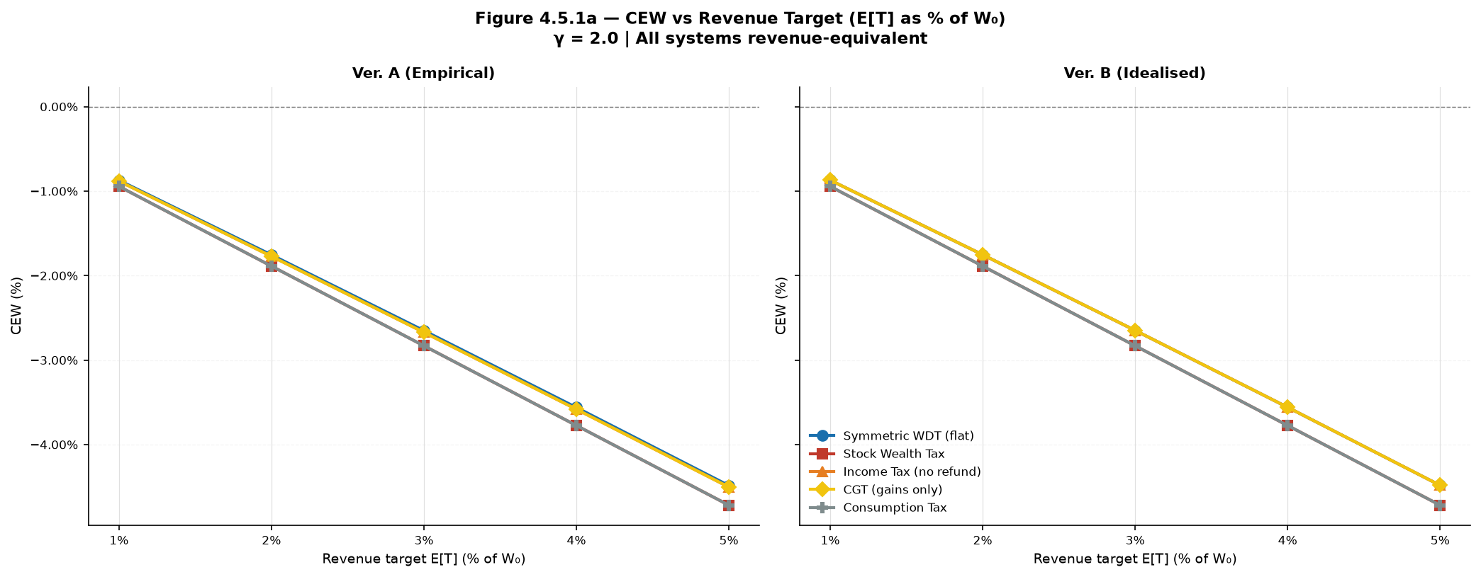
Sweeping from 1% to 5% of \(W_0\) tests whether welfare rankings are stable as the aggregate revenue burden doubles or halves from the central case. Table 12 reports CEW by system and revenue target at γ=2 for both distributions; full tables are in (WFR.A §E.1).
Table 12: CEW by System and Revenue Target (γ=2, selected targets)
| System | E[T]=1% | E[T]=2% | E[T]=3% | E[T]=5% |
|---|---|---|---|---|
| Flat WDT | −0.871% | −1.754% | −2.650% | −4.485% |
| Income Tax | −0.881% | −1.771% | −2.672% | −4.503% |
| CGT | −0.881% | −1.771% | −2.672% | −4.503% |
| Stock Wealth Tax | −0.944% | −1.887% | −2.831% | −4.718% |
| Consumption Tax | −0.944% | −1.887% | −2.831% | −4.718% |
Ver. A distribution. Revenue equivalence solved numerically at each target. Full five-target table in (WFR.A §E.1).
No ranking reversal occurs across the full 1%–5% range. The flat WDT leads income tax and CGT at every target in Ver. A; stock wealth and consumption tax sit below all accrual-base systems at every target. Welfare costs scale approximately linearly with revenue extracted — the slope is nearly constant across systems — because the underlying mechanism in each case is proportional to the rate required to hit the revenue target. A ranking that holds at 2% of \(W_0\) therefore holds at any revenue target in the tested range.
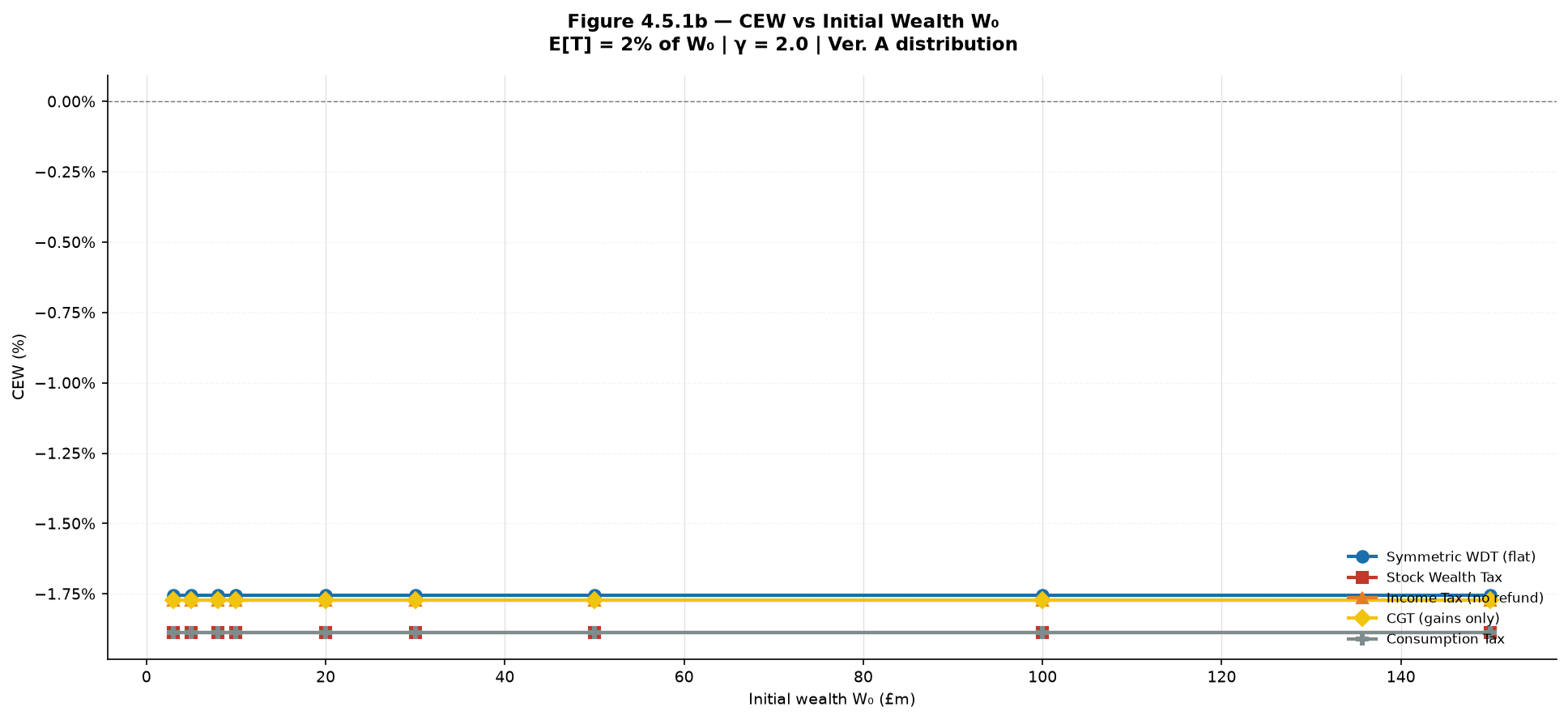
The \(W_0\)-invariance result in Figure 4.5.1b confirms a related property. Fixing E[T] at 2% of \(W_0\) and varying \(W_0\) from £3m to £140m produces flat CEW series for every system: the welfare outcome is independent of initial wealth level. The two-cluster structure from (WFR §3.1) is reproduced exactly across the full \(W_0\) range.
4.5.2 Historical Window Robustness
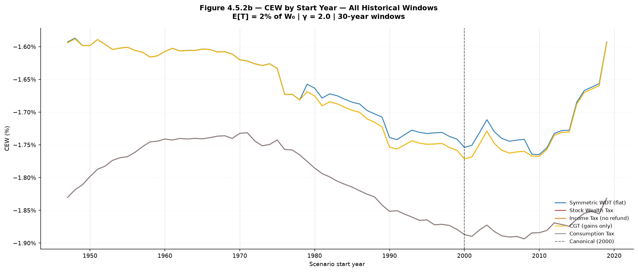
The canonical scenario is a 30-year window starting in 2000, chosen because it is the most recent non-overlapping 30-year window in the JST dataset and because it encompasses both the dot-com correction and the global financial crisis. This makes the 2000 start year a conservative choice for evaluating the WDT — its symmetric refund is most valuable precisely in windows with large negative-return episodes. Confirming that the WDT leads across the full set of historical windows establishes that the (WFR §3.1) result is not an artefact of an adversely chosen starting point.
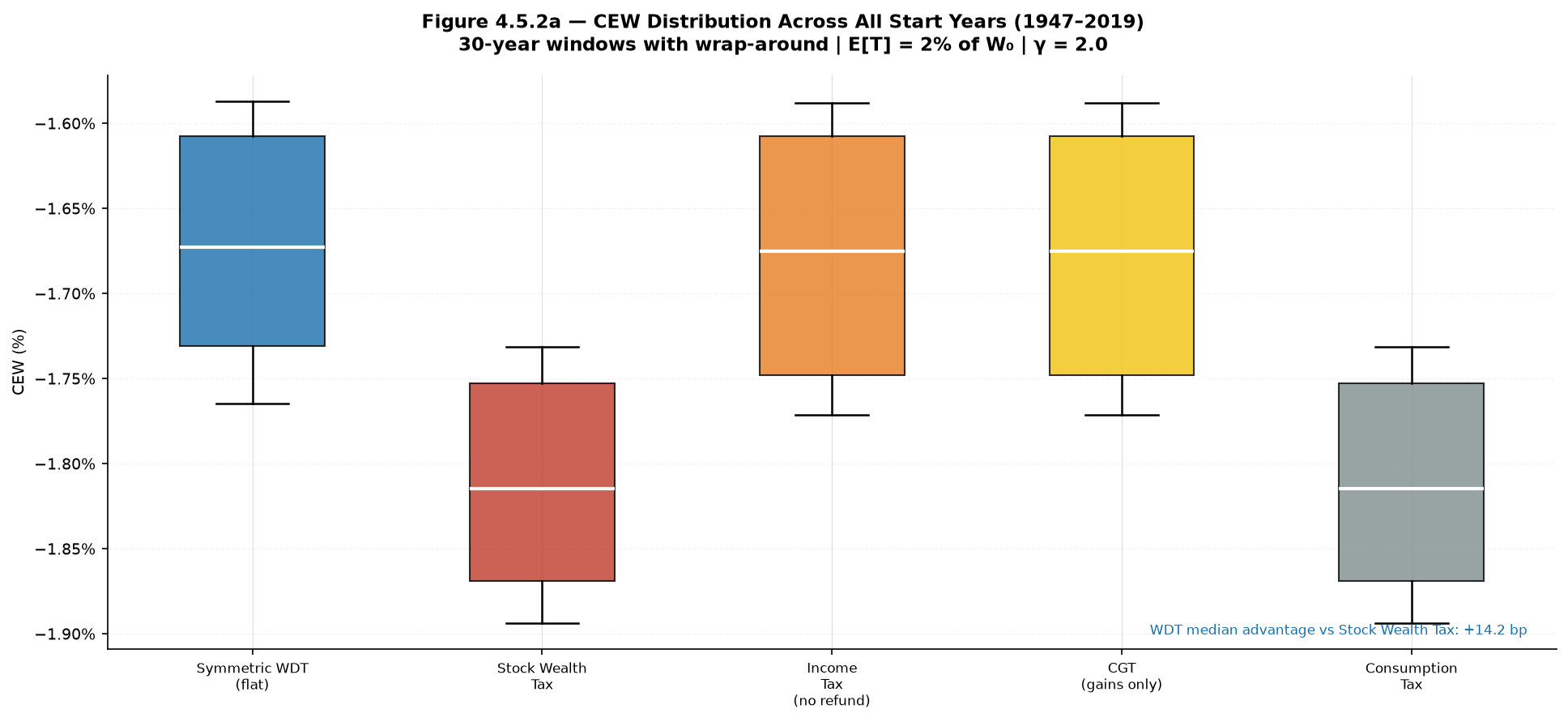
Sweep B applies the same revenue-equivalence comparison across all 73 possible 30-year windows in the dataset, from the 1947 start year to the 2019 start year (completed with wrap-around to the beginning of the dataset).
The flat WDT achieves the highest CEW of any system in 100% of the 73 historical windows. Its median CEW across windows is −1.673%, against −1.675% for income tax and CGT and −1.814% for stock wealth and consumption tax. Its worst-case CEW (−1.765%) is higher than the worst-case CEW of any competing system. The WDT’s median advantage over the stock wealth tax is 14.2 basis points — close to the canonical 2000-start result of 13.3 basis points, confirming that 2000 is not an outlier.
Table E.2.2 in (WFR.A) reports curated worst-case start years: 1972 (oil shock), 1987 (Black Monday window), 1999 and 2000 (GFC in window), and 2006 (worst LRR fill speed in the RATES analysis). The WDT advantage over the stock wealth tax ranges from 11.8 basis points (1972 start) to 14.6 basis points (2006 start). No adverse start year narrows the advantage below 11 basis points or produces a reversal.
Stock wealth and consumption tax CEW varies more across start years (spread from −1.731% to −1.894%) than WDT CEW (−1.587% to −1.765%), because the stock base collects its full levy regardless of return performance in each year of the window. The WDT’s symmetric refund moderates the worst outcomes without requiring a fortuitously timed start year.
4.5.3 Progressive Rate Parameter Sensitivity
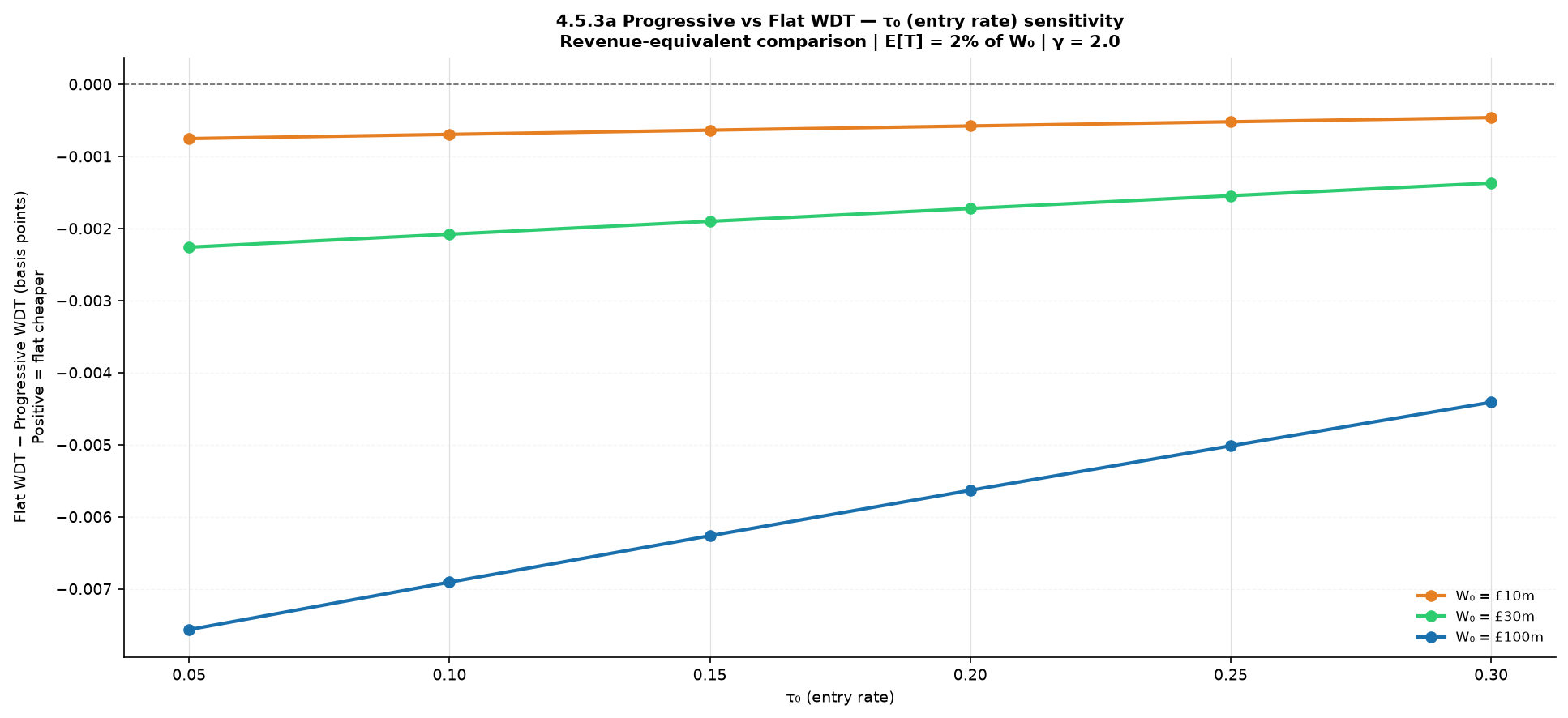
Section 4.1 established that the three D-M complications are all second-order at canonical logistic parameters, with C1 producing a flat-versus-progressive welfare gap of −0.00 basis points at the canonical test wealth. Sweep C varies each of \(\tau_0\), \(\tau_m\), \(k\),and \(W_{min}\) independently to test whether the C1 conclusion is fragile to parameter choice.
Across all four axes, the results are the same: the flat-versus-progressive welfare gap (Gap = CEW_flat − CEW_progressive, basis points) remains below 0.05 basis points in absolute magnitude across the full tested range for every wealth level and parameter combination, with one exception.
The exception is the \(W_{min}\) sweep at \(W_0\) = £10m. When \(W_{min}\) is raised to £10m — equal to \(W_0\) — the agent sits exactly at the entry threshold, the progressive schedule applies only the entry rate \(\tau_0\), and the gap turns positive (+1.74 basis points). This is not an economically meaningful exception: it requires \(W_{min}\) \(\approx\) \(W_0\), which means the taxpayer is simultaneously being assessed and sitting exactly at the threshold below which they would not be assessed at all. No other combination in the four sweeps produces a positive gap or a gap approaching 0.1 basis points.
The steepness parameter \(k\) produces the largest absolute gaps within the feasible range: at \(k\) = 0.01 and \(W_0\) = £100m, the gap reaches −0.05 basis points — two orders of magnitude smaller than the baseline welfare differences between systems. The crossing of the £100m series at \(k\) = 0.05 reflects the agent reaching the region above the logistic inflection point, where gain and refund rates reconverge near the \(\tau_m\) ceiling. That crossing occurs far outside the canonical parameter space and is noted for completeness.
The four sweeps confirm that the second-order conclusion does not rest on a fortuitous choice of canonical parameters.


5. Part III: Literature Positioning
5.1 Domar-Musgrave and Risk-Sharing
Domar & Musgrave (1944) establish the risk-sharing result for proportional taxation with symmetric loss offsets in the Quarterly Journal of Economics. When the government taxes gains and refunds losses at the same rate, the investor’s after-tax return distribution is contracted proportionally — upside and downside alike — without altering relative risk rankings. Sandmo (1977) confirms the same mechanism from a portfolio equilibrium starting point, finding that asymmetric tax treatment penalises variance directly: where losses receive no equivalent relief, investors face rising effective costs of volatile positions and underinvest in risky assets relative to what their risk-adjusted returns justify. Stiglitz (1969) formalises the conditions under which proportional taxation with full loss offset can leave the optimal risky portfolio share unchanged; King (1977) extends the analysis to show that asymmetric loss treatment raises the cost of capital for risky projects across the investment universe.
The flat symmetric WDT is a direct application of the Domar-Musgrave mechanism to a net wealth delta base. The floating-point confirmation in (WFR §3.2) is not a calibration result but a verification that the design satisfies the mathematical conditions the D-M tradition identifies.
The settled question is the risk-sharing mechanism; the open question is the welfare translation. Domar and Musgrave show that symmetric taxation avoids a specific distortion. Whether avoiding that distortion translates into welfare advantage depends on what else is true about the economy and what distortions the competing systems introduce. That translation is the subject of Part II.
5.2 Progressive Taxation and Risk Asymmetry
Vickrey (1939) identifies the rate asymmetry problem for progressive income averaging: if gains fall into a higher bracket than the one at which equivalent losses are refunded, a nominally symmetric system discriminates against risk-taking even with full loss offsets. The mechanism applies to the WDT’s logistic rate function. Section 4.1 quantifies it under the specific WDT schedule: rate differentials ranging from +0.0011 percentage points at £3m to +0.0946 percentage points at £200m, with Excess uniformly negative because the canonical population sits in the near-flat entry region of the logistic well below the inflection point. The direction of the effect is literature-supported; the magnitude and the counterintuitive negative Excess result are this paper’s contributions at these parameters. Vickrey’s diagnosis applies; his predicted direction requires the population to be operating on the steeply progressive limb of the rate schedule, which the canonical calibration does not reach.
5.3 CGT Lock-In: Literature and Model Contribution
The welfare cost of realisation-based capital gains taxation has a long analytical record. By making realisation the taxable event, CGT allows unrealised appreciation to accumulate without tax but imposes a switching cost on any taxpayer who holds an embedded gain and wants to move to a superior asset. The IMF and the OECD have documented the resulting portfolio rigidity across multiple country studies; the OECD’s 2025 analysis of capital gains tax design explicitly identifies lock-in as the primary efficiency cost of realisation-contingent systems (OECD (2025)).
Empirical literature confirms the mechanism is real and economically significant at the magnitudes the model implies. Studies of portfolio reallocation behaviour consistently find that taxpayers with large embedded gains hold them longer and switch less frequently than portfolio theory would predict without tax — and this divergence is correlated with the size of the embedded gain and the prevailing CGT rate in ways not explained by information or transactions costs alone.
WFR’s specific modelling contribution is the P(locked in) decomposition in (WFR.A §C.1): separating states where the agent does not switch because asset B is simply inferior from states where the agent does not switch despite asset B being superior because the embedded CGT liability makes switching irrational. At the reference calibration (G/V = 50%), 86.7% of locked-in probability reflects market return states where r_B < r_A. The CGT distortion proper first appears above G/V = 36.3%. This distinction is not made in the empirical portfolio literature, which has not decomposed lock-in probability in this way.
The 141–143 basis-point welfare cost at the reference calibration is the model’s result at the stated parameters. It is not an estimate of the general welfare cost of CGT lock-in in the UK economy. The mechanism is very strongly supported in the existing literature. What the model establishes is that across plausible UK parameter ranges, the welfare cost is large relative to the baseline differences between systems in Part I.
The Arachi objection requires direct treatment here. Arachi & D’Antoni (2022), in Fiscal Studies, establish that accrual taxation is not automatically welfare superior to realisation-based taxation — an accrual tax bills unrealised gains before the taxpayer has received cash from those gains, creating intertemporal consumption distortions in appreciation years. This objection applies to any accrual proposal that does not specifically address the intertemporal distortion mechanism. Section 4.2.3 establishes that the symmetric refund directly addresses the loss-year component of the Arachi critique for established taxpayers, while acknowledging that the objection applies in full at the entry margin where the lifetime contribution envelope floor binds. The engagement is structural rather than rhetorical.
5.4 Heterogeneous Returns and Concentration
Fagereng et al. (2020), in Econometrica, provide the empirical foundation for the heterogeneous-returns analysis in (WFR §4.3). Their Norwegian administrative dataset establishes persistent individual-level return heterogeneity with a cross-sectional standard deviation of approximately 8 percentage points; substantial year-to-year autocorrelation within individuals that survives controls for portfolio composition; and a positive correlation between wealth level and financial asset returns of approximately 3 percentage points between the 10th and 90th percentile, even within asset classes. A companion paper in the American Economic Review (Fagereng et al. (2016)) establishes the same persistence properties using a slightly different sample definition.
WFR’s four-tier calibration draws conservative parameters from this evidence — an outer-tier return differential of approximately 8 percentage points against Fagereng’s observed 18-percentage-point gap. The 479-fold concentration result for stock-base systems at N=30 is therefore a lower bound on what the full Fagereng heterogeneity would produce. WFR’s specific modelling contribution is the multi-decade concentration path: asking not what return heterogeneity implies at a point in time but what it implies when different tax bases either attenuate or fail to attenuate the differential compounding of persistent return differences across taxpayers. This question has not been formally examined in the existing concentration literature.
5.5 The Active Dispute WFR Enters — and Does Not Adjudicate
Guvenen et al. (2023), in the Quarterly Journal of Economics, formalise the efficiency case for a stock wealth tax over capital income taxation when returns are persistently heterogeneous. Their use-it-or-lose-it mechanism: capital income taxation concentrates the burden on productive investors who earn high returns, penalising efficient capital deployment, while a stock wealth tax falls equally on all holders of equivalent wealth regardless of return, shifting the burden toward unproductive holders and encouraging capital to concentrate with investors who earn more from it. Their model, calibrated to US data, finds a welfare gain of approximately 8% in consumption-equivalent terms from replacing capital income tax with a revenue-neutral stock wealth tax.
Gerritsen et al. (2025) (2025, Economic Journal) and Boadway & Spiritus (2025) reach the opposite conclusion from the same premise. When individuals earn persistently heterogeneous returns, positive capital income taxation can be Pareto-efficient and the optimal rate rises with the degree of return heterogeneity — the case for taxing capital income strengthens, not weakens, as return dispersion increases. Their mechanism: heterogeneous returns imply that the planner can use capital income taxes to redistribute toward low-return individuals without distorting the margin that matters, because the productive investor’s return advantage is in part a rent that taxation can extract. The Guvenen and Boadway-Spiritus papers reach directly opposing welfare conclusions from the same empirical premise and represent an unresolved dispute at the frontier of optimal taxation under return heterogeneity.
WFR does not adjudicate this dispute. Neither paper includes a delta-based accrual tax as one of the instruments under comparison. WFR introduces the delta instrument into a comparison that has been conducted across only two alternatives, which is a gap-filling contribution rather than a side-taking one. The delta base is neither a stock wealth tax nor a capital income tax: it taxes the annual change in net worth above a cost-of-capital allowance, which means a productive entrepreneur whose wealth is stable pays nothing under the delta base even if their return is high and their stock is large. Whether this property strengthens or weakens the Guvenen use-it-or-lose-it mechanism, or changes the conditions under which the Boadway-Spiritus optimality result holds, cannot be determined within the partial equilibrium framework of this paper. That analysis is the substance of a Level 2 general equilibrium extension, noted as an open question in (WFR §7.2).
Dalle Luche et al. (2026) (Review of Income and Wealth) and Garbinti et al. (2026) extend the analysis to joint heterogeneity in wealth and returns at the top of the distribution, finding that increasing returns to wealth at the upper tail have implications for optimal tax design that the Guvenen and Boadway-Spiritus frameworks do not fully capture. WFR’s contribution is to position the delta instrument in this frontier debate, not to resolve a dispute the frontier has not resolved.
WFR cannot claim that the literature establishes accrual taxation as superior to capital income taxation when returns differ: the dispute is live and the paper has no basis for adjudicating it within its partial equilibrium scope. What the paper can claim is that the existing dispute has been conducted without the delta instrument and that WFR introduces it.
5.6 Stock Wealth and Consumption Tax Equivalence
The welfare equivalence of stock wealth taxes and consumption taxes in simple lifecycle models is a well-established theoretical result. Bastani & Waldenström (2020), in the Journal of Economic Surveys, confirm the conditions under which the two systems produce equivalent welfare implications: no labour income, proportional bases, a uniform saving rate, no liquidity constraints, and CRRA preferences. The Hebous et al. (2024) IMF’s (2024) analysis of wealth tax design provides further institutional confirmation of the equivalence and the conditions under which it breaks.
WFR’s contribution is the exact numerical confirmation at both welfare (−1.8870% for both systems across all γ values) and concentration (479× for both at N=30). The exact equivalence is a model-structural property: both systems apply a fixed proportional wedge to a base that does not condition on return performance, and CRRA scale-invariance makes the welfare result independent of risk aversion. The same γ-independence that produces the welfare equivalence explains the concentration equivalence: neither system attenuates the Fagereng return differential between taxpayers, so both allow the full 8-percentage-point differential to compound unattenuated across the 30-year horizon.
The paper is precise about where the equivalence breaks. Each of the model’s simplifying assumptions, when relaxed, creates a wedge between the two systems. The equivalence result is presented as a clean finding under controlled conditions, not as a claim about the two systems’ real-world comparability.
5.7 Literature Summary
Table 11 maps WFR’s main findings against the literature on which they rest and states the drafting basis for each claim.
Table 11: Literature Map
| WFR finding | Literature basis | Drafting note |
|---|---|---|
| Flat symmetric WDT satisfies Domar-Musgrave | Domar & Musgrave (1944); Sandmo (1977); Stiglitz (1969); King (1977) | Confident assertion — WFR verifies that the delta base satisfies the mathematical conditions the D-M tradition identifies |
| D-M is a risk-sharing result, not a welfare-superiority result | Domar & Musgrave (1944) (scope of original result) | Confident assertion — the limitation is explicit in D-M; WFR restates it as framing discipline |
| Progressive schedule breaks D-M; three complications all second-order at canonical parameters | Vickrey (1939) for the underlying rate-asymmetry problem; magnitude is WFR’s own | Model contribution — direction literature-supported; magnitude and the negative Excess result are this model’s findings at this calibration |
| CGT lock-in is real and large at plausible parameters | OECD (2025) and empirical portfolio literature for the mechanism; magnitude is WFR’s own | Model contribution — the 141–143 bp figure is WFR’s at stated parameters; the mechanism and its empirical relevance are strongly literature-supported |
| P(locked in) decomposition distinguishing CGT distortion from market preference | Not previously made in this form | WFR contribution |
| Symmetric refund directly addresses the loss-year component of the Arachi objection; objection applies in full at the entry margin where the envelope binds | Arachi & D’Antoni (2022) for the objection; WFR’s structural response is its own | WFR contribution — the paper is the first to engage with this objection at the design level for a symmetric-refund accrual tax; the entry-margin qualification is WFR’s own finding |
| Fagereng return heterogeneity is persistent, large, and wealth-correlated | Fagereng et al. (2020) | Confident assertion — WFR uses their parameter estimates directly |
| 479× Great/Poor concentration for stock-base systems at N = 30 | Mechanism follows from Fagereng et al. (2020) applied to stock base; the multi-decade simulation is WFR’s | Model contribution — the concentration path is WFR’s simulation at Fagereng parameters |
| Delta base attenuates concentration; accrual vs stock is the relevant axis at N = 30 | Mechanism is WFR’s; the Fagereng foundation is established | Model contribution |
| Stock wealth tax and consumption tax are welfare-equivalent in the model | Bastani & Waldenström (2020) and IMF (2024) for the general conditions; numerical confirmation is WFR’s | Confident assertion for the equivalence conditions; model contribution for the exact numerical confirmation |
| WFR does not adjudicate Guvenen vs Boadway-Spiritus | Guvenen et al. (2023); Boadway and Spiritus (2025) | Framing statement — the paper’s gap-filling position relative to a live dispute |
6. Part IV: Synthesis and Conclusion
6.1 What the Model Establishes and What It Does Not
Three welfare objects appear across Parts I–II: individual certainty-equivalent welfare (CEW), distributional incidence of expected tax, and multi-decade wealth concentration. These are distinct. A lower CEW cost is a welfare improvement under the individual CRRA criterion this paper uses. A higher Great/Poor incidence ratio is a distributional property, not automatically a welfare improvement — whether more progressive incidence is better depends on the social welfare function, which this paper does not specify. Lower wealth concentration at N=30 under the Fagereng calibration is a structural outcome of the tax base; connecting it to welfare requires a normative argument about what concentration costs that is outside this paper’s scope. Results reported in each of the three dimensions should be read as the specific welfare object they measure, not as interchangeable evidence of overall superiority.
6.1.1 Category 1: Modelled Properties of Incumbent Systems
The model has established four findings about existing tax systems under controlled conditions at revenue equivalence. These are findings of this model at the stated parameters, not general empirical claims about real-world welfare costs. None requires the WDT to exist. A reader who rejects the WDT entirely must still account for them on their own terms.
CGT lock-in imposes a welfare cost of 141–143 basis points at the reference calibration. Once portfolio choice is endogenous and the realisation decision is modelled, CGT produces a switching wedge that costs the agent 141.22 basis points of CEW at the reference calibration (G/V = 50%, T = 5, \(\tau_{cgt}\) = 24%, Ver. A, γ=2) — growing to 162.2 basis points at G/V = 76.6% and reaching a plateau of 181.1 basis points from T = 8 years onward. The mechanism is textbook and very strongly supported in the empirical literature. The magnitude is this model’s contribution at this calibration.
Under Fagereng-calibrated return heterogeneity, the model produces 479-fold model-simulated Great/Poor concentration at the 30-year horizon for stock-base systems. Both stock-base systems levy proportionally on wealth regardless of return performance, leaving the full 8pp differential to compound unattenuated across 30 years. This is a structural property of the stock base — any system conditioning the tax on the stock rather than the return will produce the same compounding mechanism — but the 479× figure is this model’s output at these parameters, not an empirical prediction of real-world concentration under those systems.
The model produces 320-fold simulated concentration for income tax at the same horizon. Income tax conditions on gains but not on a net-return benchmark, so the gross Fagereng differential compounds without attenuation below the cost of capital. The result is worse than both WDT variants (286–288×) but substantially better than the stock-base systems (479×). The relevant comparison axis at N=30 is accrual basis versus stock base, not flat versus progressive rate.
Income tax and CGT are welfare-equivalent when the realisation rule is suppressed. The large real-world divergence between income tax and CGT operates entirely through the lock-in mechanism. The realisation rule — not the rate, not the base in isolation — is the welfare-relevant policy choice. A reform that moved from CGT to income tax without eliminating the realisation rule would not capture the welfare gain the model attributes to eliminating the lock-in distortion.
6.1.2 Category 2: Structural Properties of the WDT Independent of Implementation
The model has established five properties of the WDT that follow from the design of the delta base and the symmetric refund, independently of any implementation outcome.
Flat-rate symmetric WDT satisfies Domar-Musgrave to floating-point precision. The government participates proportionally in both gains and losses across all return states, contracting the net return distribution by the factor (1−\(\tau\)) without altering relative risk rankings. This holds at γ=1, 2, and 4 and across both return distributions. It is a structural consequence of the flat rate combined with full symmetric refunds.
The WDT eliminates realisation lock-in by construction. The switching decision between assets is not tax-relevant under the delta base: changing from asset A to asset B changes the future return stream the delta base is applied to, but does not trigger a realisation event and does not create a switching wedge. Lock-in cannot arise under the WDT by construction, not by calibration.
The lifetime contribution envelope bounds taxpayer-level lifetime refund exposure. Refund obligations cannot exceed cumulative receipts from any taxpayer whose envelope is not binding. This eliminates open-ended actuarial exposure at the individual level. The boundary condition — where the envelope binds for early entrants in loss years, as demonstrated for the Poor tier in (WFR §4.3) — creates a real initial-cohort capitalisation requirement for the SRR, not a structural funding shortfall.
The WDT is more progressive in incidence than income tax under heterogeneous returns. The delta base scales with both wealth and return differential; income tax scales with gains only. The Great/Poor incidence ratio is 6.6:1 for the flat WDT versus 3.2:1 for income tax, despite identical aggregate revenue targets. This is a structural consequence of the accrual base under Fagereng-style return heterogeneity.
The symmetric refund delivers disproportionate welfare benefit to low-return taxpayers. The Poor tier — most frequently in loss states — receives the symmetric refund in the years when it is most needed. The WDT advantage at the Poor tier is 38.1 basis points over income tax under the flat rate and 46.3 basis points under the progressive rate.
6.1.3 Category 3: What We Do Not Know
The following are real prospective costs of WDT implementation. This paper does not claim they are zero or small. Their magnitude is not currently determinable; a break-even analysis — the contribution of the companion paper EVAL — is the correct tool for evaluating whether any of them plausibly exceeds the Category 1 welfare costs the paper has established.
Valuation friction under Route D. The four-route valuation architecture (VAL) is designed to minimise friction by making declared values the legally operative basis. The empirical friction cost under real-world implementation — administrative load, professional fees, contested declarations, auction proceedings — is not quantifiable without implementation data.
Compliance and avoidance costs at scale. (BEHAV) establishes theoretical stability of the mild-overstatement equilibrium (\(\alpha\) \(\approx\) 1.1–1.5) and characterises the nine behavioural shapes from full compliance to active resistance. It does not establish the empirical compliance cost that HMRC-level implementation would generate, nor the avoidance cost at the population level once Shapes 4–6 (restructuring, timing manipulation, cross-border asset migration) are active.
Administrative learning dynamics. The speed at which an administering body develops operational competence with the Route D auction process, the declaration review system, and the settlement architecture has no direct empirical analogue. The cost of the learning period is real; Phase One is designed to generate data on it (PHASE1 §2).
Migration response. Jakobsen et al. (2020) and Agrawal et al. (2025) provide calibration ranges from existing wealth taxes, but WDT-specific migration dynamics are untested. The cross-base externality identified by Agrawal et al. (2025) — income and VAT losses approximately six times the direct wealth-tax revenue loss — is the dominant empirical qualification on all pre-behavioural revenue figures in this paper and in (RATES). Its magnitude under WDT-specific conditions is a Phase One measurement priority (PHASE1 §3).
Novel avoidance strategies specific to the symmetric refund. The mild-overstatement equilibrium (ENV §2) is the settled equilibrium for the declaration game under canonical parameters. Avoidance strategies specific to the symmetric refund — engineered losses to maximise refund exposure, basis manipulation to time loss recognition, cross-asset structuring to shift returns into refund-eligible periods — are prospective. Their magnitude depends on the legal architecture, enforcement capability, and the Rule D auction’s deterrent effectiveness.
6.2 The Comparative Question
The welfare comparison between existing systems and the WDT cannot be resolved by observing that the WDT has not been implemented. That observation establishes that Category 3 costs are unknown — it does not establish that they are large, or that they exceed the Category 1 costs the paper has measured for the systems the WDT would replace.
The correct question is: are the Category 3 prospective costs of WDT implementation plausibly larger than the Category 1 welfare costs of the systems WDT would replace?
Administrative familiarity does not answer this question. The CGT’s 141–143 basis point lock-in cost and the stock wealth tax’s 479× concentration path are not reduced by the fact that those systems are familiar.
The break-even framing translates the question into tractable form. Starting from the 141–143 basis point lock-in welfare advantage of the WDT over CGT, the question becomes: how large would each Category 3 cost have to be, individually, to offset that advantage? If the break-even for migration requires, for example, 40% of assessed taxpayers to exit the jurisdiction — far outside the range of any empirical wealth-tax response in the existing literature — then migration cannot plausibly explain away the welfare advantage. If a break-even threshold falls within a plausible empirical range, that identifies a genuine uncertainty requiring resolution before the comparison can be settled. That is EVAL’s primary contribution. WFR provides the welfare baseline EVAL’s break-even analysis will use as its starting point.
6.3 The Burden-of-Consideration Conclusion
Once tax systems are compared on their welfare consequences rather than on their administrative familiarity, the WDT cannot reasonably be dismissed without addressing the mechanisms this paper has identified and quantified.
The mechanisms are four.
Symmetric risk participation. The delta base with symmetric refund satisfies the Domar-Musgrave risk-sharing condition by construction, contracting the agent’s consumption variance below the level of every alternative tax system modelled here at revenue equivalence. The mechanism is structural — it follows from the proportional co-investment design — and is not a calibration-dependent result within this model.
Structural elimination of realisation lock-in. CGT with endogenous portfolio choice imposes a welfare cost of 141–143 basis points at the reference calibration, approximately 82 times the baseline welfare difference between systems. This cost is eliminated by construction under the WDT because the tax base does not make the switching decision tax-relevant. The symmetric refund directly addresses the loss-year component of the Arachi intertemporal consumption objection for established taxpayers; as established in (WFR §4.2.3), the objection applies in full at the entry margin where the envelope floor binds.
Concentration moderation under persistent return heterogeneity. At the 30-year canonical horizon, WDT variants reach 286–288× Great/Poor concentration versus 320× for income tax and 479× for stock wealth and consumption tax. The split is accrual versus stock base. The delta base’s conditioning on net return above a cost-of-capital benchmark attenuates the compounding of the Fagereng return differential that produces the 479× outcome under stock-base systems.
Progressive incidence from the accrual base. The WDT is more progressive in incidence than income tax — a 6.6:1 Great/Poor ratio versus 3.2:1 — because the delta base scales with both wealth and return differential. The symmetric refund delivers disproportionate welfare benefit to the low-return tier.
The model identifies several mechanisms that favour the WDT under its stated assumptions, while leaving implementation costs and general-equilibrium effects unresolved. The quantitative importance of those unresolved effects determines whether the partial-equilibrium results survive in a full welfare comparison. The relevant analytical question is: which Category 3 costs, at what empirically plausible magnitudes, would be sufficient to offset the Category 1 welfare costs the model has measured?
That question has four components. Whether the CGT lock-in mechanism operates as the model describes is a matter the empirical literature on portfolio reallocation and realisation behaviour bears on directly. Whether persistent return heterogeneity interacts with the stock base to produce concentration paths of the magnitude the model shows depends on whether the Fagereng findings extend to UK conditions — an empirical question (WFR §7.3). Whether Category 3 prospective costs of WDT implementation plausibly reach 141–143 basis points is what EVAL’s break-even analysis is designed to test. And whether any welfare cost of the WDT not identified in this paper is large enough to reverse the comparison is what Phase One is designed to reveal.
None of these questions is resolved here. The model establishes the pre-behavioural partial-equilibrium baseline. The next steps — break-even analysis in EVAL, empirical measurement in PHASE1 — determine whether that baseline survives contact with the full cost picture.
This paper does not claim the WDT is the optimal tax system. It establishes that the welfare case is coherent under controlled conditions, that it rests on mechanisms independently well-evidenced in the existing literature, and that the principal loss-year objection to accrual taxation is substantially addressed by the WDT’s symmetric design — with the entry-margin qualification stated in (WFR §4.2.3). A complete welfare comparison would require the Category 3 costs identified in (WFR §6.1.3) to be measured against this baseline. That is the work of EVAL and PHASE1. What this paper provides is a baseline against which that comparison can be conducted.
7. Open Questions
7.1 Behavioural Calibration
This paper is pre-behavioural throughout. All results assume agents respond to tax incentives only through the mechanism being tested in each section — the realisation decision in (WFR §4.2), the portfolio allocation in (WFR §3.2), the concentration dynamics in (WFR §4.3) — without modelling second-order responses such as risk-taking adjustment, labour supply, consumption timing, or strategic asset structuring. This limitation is shared with (RATES), which uses the same pre-behavioural assumption for all revenue and burden figures.
The results in this paper are therefore bounds rather than point estimates. Where WDT’s structural properties generate positive behavioural effects — the symmetric refund encouraging risk-taking, the elimination of lock-in enabling portfolio reallocation toward higher-return assets — the welfare advantage over CGT and stock-base systems would widen under a behavioural model. Where WDT’s implementation generates negative behavioural effects — migration, avoidance, restructuring — the advantage would narrow. WFR establishes the pre-behavioural welfare baseline; whether positive or negative behavioural effects dominate at calibrated parameters is the question EVAL is designed to answer.
7.2 General Equilibrium
The analysis is partial equilibrium throughout. Prices, wages, interest rates, and the aggregate capital stock are held fixed. This is the correct scope for a Level 1 paper establishing theoretical welfare properties under controlled conditions, but it leaves several general equilibrium channels unexamined.
The most consequential omission is the capital allocation effect. Under Fagereng-style persistent return heterogeneity, the choice of tax base determines not just who bears the welfare cost but whether the tax system creates incentives for capital to move toward higher-return uses. A stock wealth tax levying equally on high- and low-return wealth creates no reallocation incentive; a delta-base tax that takes more from high-return wealth and refunds low-return wealth attenuates the reallocation signal in one direction and strengthens it in another. The general equilibrium welfare effect of this channel — which is the substance of the Guvenen et al. dispute with Boadway and Spiritus discussed in (WFR §5.5) (Boadway & Spiritus (2025), Gerritsen et al. (2025)) — cannot be evaluated within the partial equilibrium framework of this paper. A Level 2 treatment would require closing the model with an aggregate production function, a capital market clearing condition, and a calibrated relationship between the return distribution and the marginal product of capital.
7.3 Implementation Cost Quantification
The five Category 3 costs identified in (WFR §6.1.3) — valuation friction, compliance and avoidance costs, administrative learning, migration response, and novel avoidance strategies — are addressed by different parts of the companion paper series at different levels of specificity: (VAL) characterises the valuation architecture and the tolerant zone but does not quantify friction at scale; (BEHAV) characterises the behavioural shapes and the mild-overstatement equilibrium but does not produce empirical avoidance cost estimates; (CLOSE) designs the departure settlement mechanism but does not estimate migration response; (PHASE1) specifies the measurement framework through which Phase One implementation would generate the first empirical data on all five costs simultaneously.
WFR establishes the welfare advantage at the pre-behavioural level. EVAL’s contribution is to test each Category 3 cost against that advantage using a break-even framework: for each cost, what magnitude would be required to offset the 141–143 basis point lock-in welfare advantage? If a break-even threshold is empirically implausible given the existing literature on analogous wealth tax systems, that cost cannot explain away the welfare advantage. If a threshold falls within an empirically plausible range, that is a genuine open question that Phase One is designed to resolve.
7.4 Progressive WDT Advantage at Longer Horizons
The N=30 concentration result shows a near-equivalence between flat and progressive WDT at the canonical horizon: 286.3× versus 288.1×. The finding that the relevant axis at N=30 is accrual versus stock base, not flat versus progressive rate, follows from the logistic schedule operating in the near-flat entry region across the tested wealth levels for 30 years. The progressive advantage is real — it is present in the CEW comparison (Table 9) and in the incidence ratios (Table 10) — but on the concentration metric it requires a longer horizon to compound into a visible differential between the two WDT variants.
The N=73 concentration extension — running the full 1947–2019 historical sequence chronologically, with the aggregate rates from (WFR §4.3) carried forward unchanged rather than re-solved — confirms this expectation, and shows the advantage emerging earlier than the canonical window alone would suggest. Progressive WDT’s Great/Poor ratio first drops below flat WDT’s in 1971, less than 25 years into the sequence, and the gap widens sharply from there: by 2019, flat WDT reaches 3,173.2× against progressive WDT’s 177.8×, an eighteen-fold difference (WFR.A §F.3; Figure F.1). The mechanism is the one the logistic geometry predicts: as the Great tier’s wealth compounds past the schedule’s inflection point, its effective rate rises toward \(\tau_m\), while the Poor tier — whose losses frequently fall below \(W_{min}\) or close to the entry rate — continues to be taxed near its floor. The resulting attenuation is concentrated almost entirely at the top of the tier structure rather than spread across it: the Great/Ok ratio falls from 336.1× under flat WDT to 18.5× under progressive, while the Ok/Poor ratio is essentially unchanged (9.4× vs 9.6×) (WFR.A §F.4; Figure F.2). The progressive schedule’s long-horizon concentration advantage is a top-tier effect, not a general compression of the tier structure.
This result does not contradict the N=30 finding above, and the two should be read as different windows rather than competing estimates. (WFR §4.3)’s canonical scenario starts in 2000 and, under wrap-around rotation, its first 30 years are a different ordering of the same 73 annual observations than the plain 1947–1976 span examined here — not a truncation of the same sequence. That progressive WDT sits on opposite sides of flat WDT in the two windows (+1.8× at the 2000-start N=30; already −1.3× and falling by 1971 in the chronological run) reflects which years fall early in each ordering, not an inconsistency in the model. It is also a scope reminder: unlike the N=30 comparisons in (WFR §4.5.2), which are tested across all 73 possible start years, the N=73 result is a single deterministic run over one historical ordering — the only ordering available at that horizon, since a 73-year window has nowhere left to rotate to. It establishes that the progressive WDT’s concentration advantage does emerge well within the observed historical record; it does not establish that 1971, specifically, is a horizon the WDT could be relied on to reach regardless of when the tax began. Confirming the crossover’s robustness to start year is a natural extension once the N=73 machinery generalises to arbitrary starting points, and is left for future work.