The Wealth Delta Tax: Valuing Wealth
Wealth Delta Tax, wealth taxation, accrual taxation, wealth valuation, self-assessment, asset valuation, illiquid assets, valuation incentives, tax avoidance, tax compliance, Harberger taxation, self-assessed valuation, declaration incentives, unrealised gains
Revision History
| Revision | Date | Details |
|---|---|---|
| 0.01 | 05 June 2026 | First Draft |
| 1.00 | 15 August 2026 | Published to website |
| 1.01 | 20 August 2026 | §9 updated to incorporate privacy election as upstream mechanism determining register content (GOV.B §B.4.7); cross-reference updated from GOV §5.3 to GOV.B §B.4.6–B.4.7; register inflation consequence of mild-overstatement equilibrium added; disclaimers section unchanged |
| 1.02 | 29 August 2026 | §11 restructured to distinguish three Route D auction pathways (corrective, voluntary hard-reset, inheritance) with separate tax treatment for each; corrective over-declaration arm added with no-refund basis-correction rule; no-bid outcome resolved as zero-basis reset with no professional fallback; taxpayer non-notification rule stated explicitly; lock-point at sealed estimate submission added; §6.4 updated with lock-point rule and corrective/voluntary distinction; §6.5 updated with symmetric refund treatment on inheritance downward discovery; §4.4 updated to reference three-pathway architecture |
| 1.03 | 30 August 2026 | TW refined to TW_settled throughout (post-sale oscillation now included in terminal figure); §5.2 updated with C.11 decomposition result and Figure 5.3 (mechanism decomposition and dilution surface); §7.1 updated with Figure 7.3 (TW_settled advantage across (g, N) surface) and present-value caveat; old Figures 7.3–7.5 renumbered 7.4–7.6; §7.3 updated with per-\(\alpha\) TW_settled peak values and C.11 citation; §7.4 C.6 figures corrected to match VAL.A Table C.6 (93.78% and 88.30%); §15 conclusion updated with C.11 decomposition sentence |
| 1.04 | 31 August 2026 | §7.1 caveat paragraph on TW_settled surface replaced with two-regime PV analysis and Figure 10 (C.12 nominal vs NPV-adjusted heatmap); §7.3 paragraph added on risk-aversion-driven equilibrium at \(\alpha\) \(\approx\) 1.1 and asymmetric refund protection under valuation uncertainty; §15 conclusion updated with C.12 sentence; (VAL.A §C.12) added. |
| 1.05 | 31 August 2026 | Abstract, §5.2, §7.1, §7.3, §9 updated to correct the mild-overstatement equilibrium claim throughout: the nominal TW_settled advantage (C.11d) does not survive NPV adjustment (C.12) and is not a genuine economic return to overstatement; the correct equilibrium rationale is refund-protection asymmetry under valuation uncertainty (\(\alpha\) \(\approx\) 1.1 risk-aversion argument from §7.3), not a wealth-maximising strategy. All claims of a “stable TW advantage” from mild overstatement replaced with accurate characterisation. |
| 1.06 | 11 September 2026 | §5.2, §7.1, §7.2, §7.3, §7.4, §14.2 updated to align figure captions and prose with actual figure content: (i) N = 30 confirmed as canonical throughout — figures are correct; (ii) Figure 7.1 prose rewritten — motivation line (gold dashed) does not exist in the figure; right panel described as N-crossing cost profile in £m rather than percentage advantage erosion; crossing values (N$$22, 21, 20, 20) taken from figure annotations; (iii) Figure 7.2 prose corrected — historical series is 2000 start year (mean g=6.0%), not 2006; the two series do not run nearly identically at overstater \(\alpha\) values; (iv) Figure 7.3 prose corrected — canonical intersection values updated to N=30 table values (2.4pp for \(\alpha\)=1.2, 6.0pp for \(\alpha\)=1.5 from VAL.A §C.11.4); PV discount factor corrected to 23p/£ at year 30; C.12 reversal values updated to N=30 (−0.91pp→−0.29pp for \(\alpha\)=1.5 at g=0.4%; −1.66pp→−0.04pp at g=5.9%); (v) Figure 7.4 prose extended to describe both constant-g and 2000 historical series line families visible in the figure; (vi) Figure 7.5 prose and caption corrected — inflection at g$\(19.1% not ~17%; plateau ceiling values corrected to those shown in the figure; (vii) Figure 7.6 prose and caption corrected — figure has one panel only; right-panel bar chart description removed; first-reversal values taken from figure annotations; (viii) §14.2 plateau inflection reference updated. | | 1.08 | 20 September 2026 | Crosslinks added: §13 extended with three-instrument SWF overview pointing to (GOV.B E.3) bridging facility and (CORP 6) corporate equity settlement facility; §14.1 extended with reciprocal pointer to (WFR 6.1.3) Category 3 cost list | | 1.07 | 12 September 2026 | Abstract, §7.1, §7.3, §9, §14.2, §15 reframed throughout: (i) tolerant zone (\)$ \(\approx\) 0.8–1.5) promoted as the primary result — the mechanism creates a broad forgiving centre with genuine penalties only at the tails; (ii) the mild upward declaration bias (\(\alpha\) \(\approx\) 1.1) characterised as a conditional model-implied behavioural prediction driven by refund-protection asymmetry under valuation uncertainty, not as a ‘population equilibrium’ or dominant strategy; (iii) the overstatement side of the tolerant zone (\(\alpha\) = 1.2, 1.5) characterised as illustrative points within the zone, not as evidence for a wealth-maximising equilibrium; (iv) §7.1 rewritten to lead with the three-layer structure (tolerant zone → tail penalties → asymmetry within the zone) rather than payoff-profile framing; (v) §7.3 corrected on C.1 boundary: at N=30 all four overstater levels cross into nominal net-cost territory above g$$7%, including \(\alpha\)=1.2 and \(\alpha\)=1.5, contrary to the prior stale claim that they stayed negative across the full tested range; (vi) ‘population equilibrium’ language replaced throughout with ‘model-implied behavioural centre’ or ‘predicted mild upward declaration bias’. |
Abstract
The standard objection to any mark-to-market wealth tax is that illiquid assets cannot be accurately valued every year. This paper argues the objection is directed at the wrong problem.
The WDT does not require annual precision. It requires that declared values carry real consequences. A taxpayer who declares a private company at a given figure has established that figure as the recognised basis from which all future changes are measured. If the company later sells at a higher price, the gap between declared basis and realised price enters the tax base in the year of sale. Undervaluation defers tax rather than eliminating it. The state’s task is to enforce the consequences of the declaration — not to certify whether the declaration was correct. Valuation accuracy ceases to be a necessary condition of tax administration.
The framework operates across four routes defined by whether an asset is fungible or non-fungible, and whether it is professionally valued or self-declared. Professional routes shift valuation risk to the valuator. Self-declaration routes shift it to the taxpayer, attaching consequences to whatever figure the taxpayer commits to. For fungible assets, settlement in kind at the declared price creates a direct compounding cost to understatement without requiring audit. For non-fungible assets, taxation is deferred to realisation, where an observable market value exists.
The simulations in (VAL.A §C) show that this architecture is not easily exploited. At canonical parameters, a broad range of declaration ratios produces lifetime tax outcomes close to honest declaration — the tolerant zone. This is a design feature, not a gap in enforcement. Within the zone, consequences are asymmetric: understatement reduces refund protection in bad years while overstatement preserves it, giving risk-averse taxpayers a modest incentive to declare slightly above their central estimate. Beyond the zone, penalties at both tails are real and accumulating.
The remaining questions are empirical. Assessment window elections, behavioural responses, and premium calibration all require Phase One data. The valuation architecture exists to maintain a credible tax base; (RATES) demonstrates that revenue properties remain robust without assuming declaration precision.
Glossary
Acquisition basis: The recognised value of an asset at the point it enters the taxpayer’s WDT net worth calculation. For existing wealth at system entry, this is the grandfathered declaration. For subsequently acquired assets, it is the value at the date of acquisition.
Assessment window premium: The charge paid by taxpayers who elect an assessment window longer than one year. It has two components: a deferral charge reflecting the time value of delayed settlement, and a flexibility levy representing the state’s share of the valuation cost saving the taxpayer captures by assessing less frequently. The premium is symmetric: where delayed assessment produces a refund, the taxpayer receives an equivalent upward adjustment.
Assessment window: The interval selected by the taxpayer between formal assessment events. Available windows are one, two, three, five, and seven years. Annual reporting obligations continue regardless of window selected.
Declared value: The value a taxpayer submits for an asset. For automatically priced assets, the declared value is determined by market price. For professionally valued assets, it is determined by the certified assessment. For self-declared assets, it is determined by the taxpayer’s own submission.
Deferral charge: The component of the assessment window premium that compensates the state for the time value of delayed settlement. It accrues from the date each liability falls due.
Delta: The change in net worth across the assessment window, or the rolling average of that change. Positive deltas generate tax liabilities. Negative deltas generate refund entitlements.
Fungible asset: An asset that can be fractionally transferred without losing its character, primarily company equity, fund units, and partnership interests.
Flexibility levy: The component of the assessment window premium that represents the state’s share of the valuation cost saving the taxpayer captures by electing a longer window. It scales with window length.
Grandfathered wealth: Net worth existing at the point a taxpayer enters the WDT system. No WDT is owed on grandfathered wealth. The taxpayer’s entry declaration establishes the recognised basis for future delta calculations.
Hard basis reset: Voluntary settlement of a Route D liability using an auction to establish market value, rather than self-declaration. The auction price becomes the new recognised basis. The mechanism is the same as the inheritance auction, applied at the taxpayer’s election.
Inheritance auction: The price-discovery mechanism triggered when a Route D asset passes to an heir. The asset is offered at public auction to establish a market value. That auction price becomes the realisation value for WDT purposes. The heir may retain the asset by paying the WDT liability calculated on that basis. If the estate does not pay, the asset is sold at the auction price and the liability is settled from proceeds.
Net worth rate: The marginal WDT rate applicable to the taxpayer, determined by their total declared net worth at the point of formal assessment.
Non-fungible asset: An asset that cannot be fractionally transferred without destroying or materially changing it. Houses, art, jewellery, collectibles, and similar assets fall here. Routes B and D apply to non-fungible assets.
Realisation event: A transaction or circumstance that produces an observable market value for an asset, including arm’s-length sale, public auction, and the inheritance auction process. For Route D assets, the realisation event is the point at which the WDT liability is calculated and settled.
Soft basis reset: Voluntary settlement of a Route D liability using a taxpayer self-declaration to establish the new recognised basis. The taxpayer declares a current value, pays the WDT liability on the gain from entry basis to that value, and the basis resets. The Route D auction mechanism remains available for egregious declarations.
References throughout this paper to (VAL.A §A) through (VAL.A §F) refer to sections of the mathematical and simulation companion (VAL.A): (VAL.A §A) (mathematical model and propositions), (VAL.A §B) (simulation methodology), (VAL.A §C) (simulation tables), (VAL.A §D) (mechanism cases), (VAL.A §E) (route specification tables), and (VAL.A §F) (annual reporting requirements). Worked examples tethered to this paper’s five claims are in (VAL.B), with each example lettered (VAL.B §J) through (VAL.B §O) to match the claim it illustrates.
1. The Valuation Problem
Every serious proposal in the Haig-Simons tradition runs into the same objection: how do you value a private company annually? The question has force. Listed equities have continuously observable prices; the assets through which the largest wealth concentrations are held — controlling stakes in private companies, founder equity, family enterprises — do not. A private company one valuator prices at £80 million another might defensibly price at £120 million.
The problem is compounded by incentive structure. The professional’s primary client relationship runs to the taxpayer whose assets are being assessed, creating systematic pressure on methodology through client relationships, hiring patterns, and professional norms shaped by the population the profession most regularly serves. The Pereira Gray (2021) identified exactly this pattern in real estate investment valuation; its diagnosis applies with at least equal force here.
Prior mark-to-market proposals acknowledged the problem without resolving it. Shakow (1986), Batchelder & Kamin (2019), and Avi-Yonah & Mazzoni (2019) each identify the valuation difficulty as unresolved or as a necessary precondition with no design solution. What these approaches share is a common assumption: that the primary challenge is discovering an objectively correct value, and that the tax system cannot function until that discovery is made. For many economically significant assets, no such value exists. But the assumption itself is wrong.
The WDT does not solve the epistemic problem of determining the true value of an illiquid asset. It solves the administrative problem created by requiring the state to determine that value as a precondition of taxation. Under conventional mark-to-market proposals, the logical structure runs: true value → state determines or estimates value → tax liability. The state must certify a number it cannot directly observe. Under the WDT’s self-declaration routes, the structure is different: declared value → legally recognised basis → consequences determined mechanically through subsequent deltas, settlement, and realisation. The state does not need to establish whether the declaration was correct — only to enforce the consequences of the declaration the taxpayer made. Valuation accuracy ceases to be a necessary condition of tax administration.
This reframing has a precise boundary. The WDT still requires professional valuation for Routes A and B, still operates Route D auctions, still maintains valuation bodies and a valuation code. For self-declaration routes, the state’s enforcement task changes category: from continuously adjudicating the correct value of every illiquid asset to enforcing declaration commitments, ownership records, and settlement rules. Those are considerably more tractable problems.
The question then becomes: under what conditions does a system of declaration commitments remain strategically stable? The answer turns on a specific feature of the WDT’s tax base. Because the WDT taxes changes in net worth rather than the stock itself, a declared value establishes a recognised basis from which future changes are measured. A taxpayer who declares a private company at £50 million when it is worth £70 million pays less tax at the assessment date, but the recognised basis is now £50 million. When the company later sells for £120 million, the taxable delta in the year of sale is £70 million. Undervaluation defers tax rather than eliminating it, and the deferral advantage narrows as the asset grows.
The simulation results in (VAL.A §C) quantify the magnitude and shape of these incentives across growth rates and holding periods. They are supporting evidence that the declaration-commitment architecture is not easily exploited — not the foundation on which the valuation solution rests. The foundation is institutional: declared values carry legally operative consequences regardless of whether they are correct. The simulations establish that those consequences are sufficiently structured to make systematic gaming unattractive under realistic parameters. Honest declaration is the only strategy that does not require the taxpayer to be right about the future to avoid a penalty. Each directional bet, whether low or high, produces a cost if the bet turns out wrong.
2. Asset Classification
The valuation problem differs by asset type. The WDT uses a two-dimension classification: whether an asset is fungible or non-fungible, and whether it is professionally valued or self-declared.
2.1 Automatically Priced Assets
Listed equities, government bonds with observable prices, exchange-traded funds, cash deposits, and money market instruments are assessed at market price on the assessment date. Standard accrued interest conventions apply to bonds; foreign cash converts at spot rate on the assessment date.
2.2 Fungible Assets
Fungible assets can be fractionally transferred without destroying the nature of the underlying holding. Company equity is the primary case: a founder who owns 60 per cent of a company can transfer 2 per cent to a third party without affecting the remaining 58 per cent. Fund units, partnership interests, and similar instruments share this property. Because fungible assets can be fractionally transferred, the WDT can settle liabilities in kind by taking a proportional equity interest at the declared value — the foundation of the self-balancing mechanism described in (VAL §5).
2.3 Non-Fungible Assets
Because fractional transfer is impossible, the WDT cannot settle non-fungible asset liabilities in kind. Settlement must be in cash. This has direct implications for the deterrence mechanism, which operates differently from the fungible case.
2.4 Why Periodic Valuation and Audit Are Insufficient
Increased professional valuation and audit requirements do not eliminate the underlying difficulty: private asset valuations remain estimates rather than observable prices, and repeated valuation disputes create administrative costs without proportionate benefit. The challenge is not detecting inaccurate declarations; it is creating a mechanism where inaccurate declarations do not create persistent advantages. The WDT addresses this by changing the role of valuation within the tax system.
3. Assessment Windows
3.1 Annual Reporting and Formal Assessment
The WDT separates two functions that have historically been conflated: ongoing monitoring, which is annual, and formal assessment with settlement consequences, which is a taxpayer election.
Annual reporting is mandatory for all taxpayers. Each year, taxpayers submit to the Administrator verification of a return specifying asset ownership, estimated current values, material changes affecting value, acquisitions and disposals, significant financing events, and changes in beneficial ownership. Annual reports are the primary fraud detection and ownership tracking instrument.
Formal assessment occurs at the end of the taxpayer’s selected assessment window: the delta is calculated, the tax liability or refund is determined, and settlement occurs according to the rules of the applicable route. So long as the assessment window premium compensates the state for timing, the total economic outcome is equivalent to annual formal assessment.
3.2 Available Assessment Windows
Taxpayers may elect one of five assessment windows: one, two, three, five, or seven years. The window applies to the taxpayer’s whole portfolio and is fixed for a given election period. Taxpayers may apply to change their window at the end of an assessment cycle, subject to a minimum holding period in the current window.
Multi-year intervals stagger assessment events across the taxpayer population and reduce the risk of synchronised demand placing pressure on valuation capacity or creating distortions in markets for illiquid assets. The state has a preference for annual assessment, which maximises accuracy, revenue timing certainty, and oversight. Longer windows are an offer the state extends, not a facility it promotes.
Route D assets do not accrue periodic liabilities during the holding period and so do not operate within the elected assessment window in the usual sense. They remain subject to annual reporting. The elected window governs formal assessment and settlement for all other assets in the portfolio.
3.3 Borrowing and Net Worth
Borrowing does not increase net worth. A loan increases both assets and liabilities by the same amount, producing no delta. The WDT does not treat borrowing as a realisation event and does not use lender valuations to update the recognised basis.
4. The Four Valuation Routes
The valuation and settlement design operates across four routes defined by two variables: whether the asset is fungible or non-fungible, and whether it is professionally valued or self-declared. Taxpayers may generally elect either route for a given asset, subject to any asset-class restrictions specified in the Valuation Code.
A taxpayer with a mixed portfolio runs multiple routes simultaneously. The routes do not interact. Each portion of the portfolio follows its own route from valuation through to settlement, and the liability from each is settled separately under that route’s rules. Settlement must match the valuation route that produced the liability.
The Route D auction mechanism (VAL §11) is the backstop for egregious self-declarations on Route D. It depends on occasional triggering for its deterrent effect and is not a routine enforcement tool.
| Professional valuation | Self-declaration | |
|---|---|---|
| Fungible | Route A | Route C |
| Non-fungible | Route B | Route D |
Table 4-1: Summary of Valuation Routes
Full route specifications, including settlement mechanics, premium treatment, and worked illustrations, are in (VAL.A §E).
4.1 Route A: Professional Valuation of Fungible Assets
Route A applies to fungible assets — company equity, fund units, partnership interests — assessed by independent professional valuation through competitive tender at the end of the assessment window. Valuation risk sits with the valuator: a valuator whose assessment is overturned in independent review loses their entire engagement fee. Settlement is in cash or professionally valued assets. No self-declared assets may be used in settlement.
4.2 Route B: Professional Valuation of Non-Fungible Assets
Route B follows the same professional structure as Route A for non-fungible assets. The key structural difference is deferred settlement: where the taxpayer does not settle immediately, the liability accrues to a running deferred balance carrying the deferral charge, secured as a lien against the asset. Settlement is forced at every change of ownership. Route B carries a lien because periodic professional assessment generates real periodic liabilities that must remain collectable; Route D, which accrues no periodic liability, requires no lien during the holding period.
4.3 Route C: Self-Declaration of Fungible Assets
Route C allows taxpayers to declare their own value for fungible assets with a brief methodology description. No professional certification is required. In exchange for that flexibility, valuation risk sits entirely with the taxpayer, and settlement must be in kind: the WDT liability is settled by transferring a proportional interest in the asset at the declared value. Cash settlement is not available.
The must-transfer requirement is the self-balancing mechanism. A taxpayer who understates transfers equity at an underpriced figure; the state’s acquired stake then appreciates at the true rate. This creates a direct and compounding cost to understatement that does not depend on audit or enforcement. Route C’s must-transfer settlement creates continuous active self-correction through dilution; no auction backstop is needed or available on this route. The full mechanics are in (VAL §5).
4.4 Route D: Self-Declaration of Non-Fungible Assets
Route D covers non-fungible assets held under self-declaration. No periodic formal assessment occurs and no liability accrues during the holding period. Annual reporting obligations continue throughout, serving fraud detection and ownership tracking, but do not generate settlement obligations.
The entry basis is self-declared and grandfathered. Settlement occurs at realisation only, calculated as the marginal rate applied to the full gain from entry basis to realisation value. This deferral to realisation is not a concession to illiquidity; it is the only coherent design for assets that cannot be fractionally transferred, as (VAL §6) argues.
A taxpayer who wishes to crystallise their Route D liability before a forced realisation event may do so through a soft basis reset (self-declaration of current value) or a hard basis reset (auction-established price discovery), described in (VAL §6.4). The Route D auction mechanism operates across three distinct pathways — corrective, voluntary, and inheritance — each with its own trigger and tax treatment, specified in full in (VAL §11).
5. The Self-Balancing Mechanism: Fungible Assets
The self-declaration route for fungible assets creates incentives for accurate reporting through the consequences of the declaration itself, rather than through professional verification or state audit. Two distinct cost mechanisms operate, each targeting a different direction of error. Understatement is deterred through equity dilution: a taxpayer who declares below true value transfers equity at that price, so the state acquires an underpriced position that appreciates at the true rate. Overstatement is deterred through rate bracket effects: inflating the declared net worth pushes the portfolio into a higher marginal rate band, raising liabilities for as long as the overstatement is maintained. Proposition 2 in (VAL.A §A.5.2) shows this cost increases with the rate escalation parameter k.
At RATES-aligned parameters, the cost of misstatement is directionally consistent and economically material across the tested range. Declaration strategy differences across growth rates are in (VAL.A §C.1); the interaction between \(k\) and terminal net worth across strategies is in (VAL.A §C.5). Limitations are addressed in (VAL §7.4).
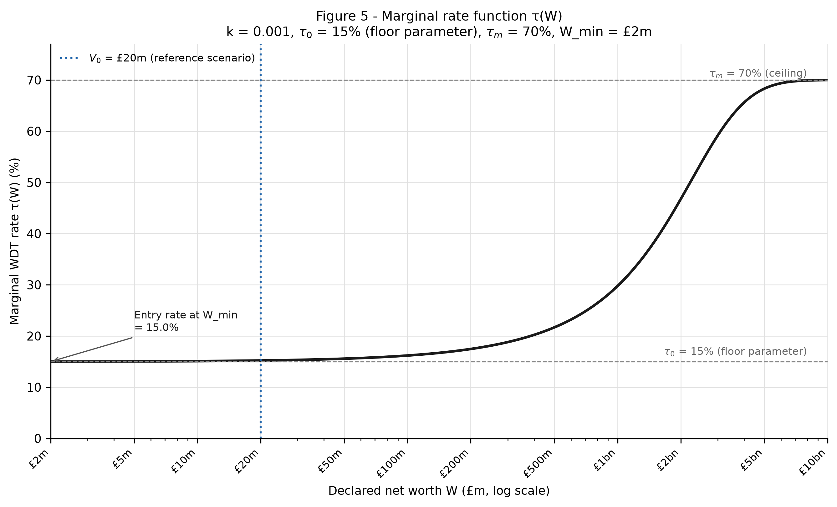
Figure 5 shows the rate function at canonical parameters. The entry rate at \(W_{min}\) = £2m is 15.0%; it remains at 15% from the threshold to approximately £200m, before rising steeply through £500m and approaching the 70% ceiling at billion-pound scale. The reference scenario at \(V_0\) = £20m sits on the flat portion of the curve. Rate bracket effects are modest at entry-level net worth and grow powerful only at very large declared bases, which explains why mild overstatement carries limited bracket penalty and aggressive overstatement faces a real one.
5.1 The Grandfathering Baseline
At entry into the WDT system, existing wealth is grandfathered. A taxpayer entering the system with a £20 million company stake owes no immediate tax regardless of what value they declare; no change in wealth has yet occurred. The entry declaration establishes the recognised basis from which all future deltas are calculated and determines the taxpayer’s marginal rate bracket at the next formal assessment.
5.2 The Must-Transfer Rule
For fungible assets on the self-declaration route, settlement must be in kind. The taxpayer transfers a proportional equity interest at their declared value. Cash is not available.
The declared price is not merely a valuation. It is a transaction price the taxpayer is prepared to stand behind. A taxpayer who declares a company stake at £100 million is saying: the state’s claim against this asset will be settled at £100 million. If that figure is below true value, the state acquires equity cheaply and participates in the subsequent appreciation. The state does not need to know whether £100 million was the correct valuation — the consequence of the declaration is the same regardless. This is the mechanism through which the WDT removes the state’s need to certify self-declared asset values: the declaration itself becomes economically operative, and its accuracy or inaccuracy resolves through subsequent delta mechanics rather than through state adjudication.
A taxpayer who declares at £100 million when the stake is worth £200 million pays lower tax but transfers equity at that lower price. The state’s acquired stake then appreciates at the true rate. The deterrence is strongest where it matters most: the faster the company grows, the more expensive the understatement becomes. Simulation results across growth rates and holding periods are in (VAL.A §C.5) and (VAL.A §C.8).
Overstatement works differently, and the outcome depends on degree. All figures below use TW_settled — terminal net worth after the post-sale tax or refund oscillation, the correct measure of lifetime outcome once the sell-year basis reconciliation is included. The nominal TW_settled decomposition in (VAL.A §C.11) shows that the inflated basis generates a sell-year refund entitlement that exceeds the f_N erosion cost and post-sale damping cost by approximately 6:1 at canonical parameters. However, this nominal advantage does not survive discounting: (VAL.A §C.12) shows that once all tax cash flows are discounted at ρ = 5%, the apparent advantage compresses sharply or reverses throughout the low-growth band where it nominally exists, because periodic outflows are real early money while the sell-year refund is inflated late money. The mild-overstatement nominal advantage is a timing artefact rather than a genuine economic return. Aggressive overstatement (\(\alpha\) ≥ 1.8) faces an additional contemporaneous structure: the bracket penalty dominates in the \(g\) \(\approx\) 9–17% corridor containing the historical mean, and the nominal TW_settled advantage is bounded near 13% at \(\alpha\) = 2.0 regardless of how far the declaration is pushed, because the rate function saturates. The full matrix is in (VAL.A §C.9) and (VAL.A §C.5).
Figure 5.2a maps the C.1 metric across the full declaration-ratio and growth-rate grid at N = 30 and \(V_0\) = £20m. Red cells indicate strategies where the taxpayer ends up paying more than honest declaration; blue cells indicate strategies where they pay less. Severe understatement is consistently red across growth rates. Mild overstatement is persistently blue from low to high growth. Aggressive overstatement (\(\alpha\) ≥ 1.8) shows a band of red at moderate growth before returning to blue at high growth, the growth-corridor pattern described above.
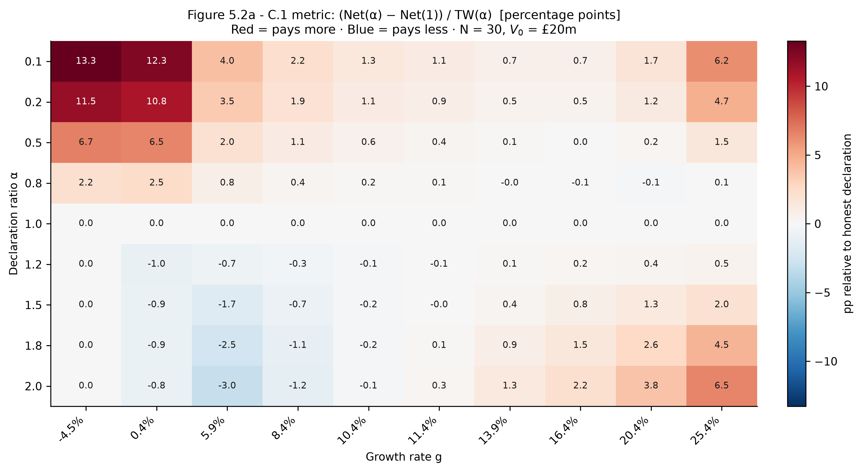
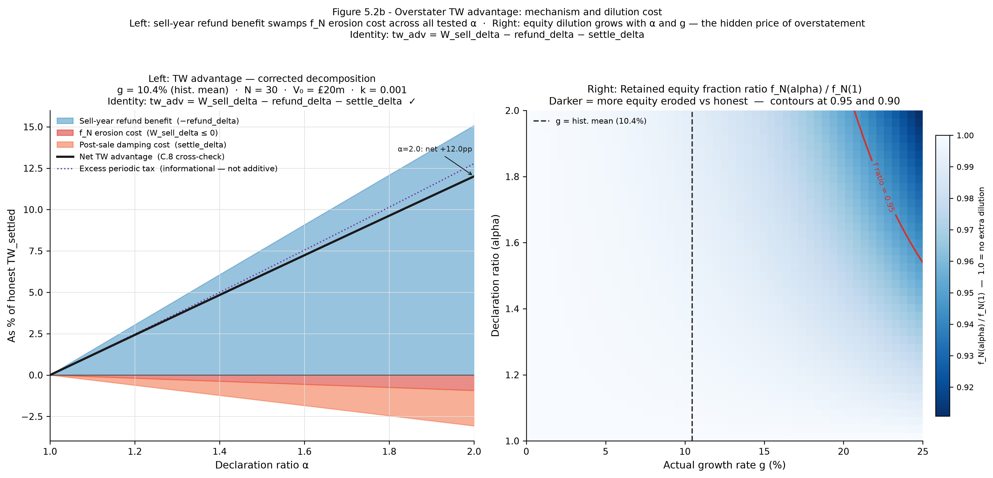
Figure 5.2b decomposes the nominal TW_settled figures into their three mechanical components. The left panel shows that the sell-year refund benefit (blue) exceeds the f_N erosion cost (salmon) and post-sale damping cost (orange) across all tested \(\alpha\), with the net nominal TW_settled figure (black line) rising to approximately +12pp at \(\alpha\) = 2.0. This decomposition explains the mechanism but not its economic significance: as (VAL.A §C.12) and Figure 10 establish, the nominal advantage does not survive discounting because periodic outflows precede the sell-year refund by the full holding period. The right panel maps f_N(\(\alpha\)) / f_N(1) across the (\(\alpha\), \(g\)) surface: darker shading indicates more equity eroded relative to the honest declarer, with the 0.95 and 0.90 contours showing where dilution becomes material.
5.3 Delta Continuity at Realisation
When a fungible asset is sold or transferred, the gap between the recognised basis and the value at transfer enters the tax base in that year. No prior declarations are reopened. A taxpayer who declared a private company at £50 million across a five-year window and sells it for £150 million recognises a taxable delta of £100 million in the year of sale, regardless of the declaration path taken during the holding period.
6. Non-Fungible Assets and Realisation
6.1 Why Periodic Accrual Is Not Workable for Non-Fungible Assets
Route D has no periodic delta calculation; the tax calculation is deferred to the realisation event. Accepting periodic self-declarations as the basis for cash liabilities has a specific problem: understatement generates a timing advantage that deferral charges cannot reliably eliminate, because the charge is calibrated against the declared amount rather than the true amount. And fractional transfer of a non-fungible asset is not possible, so Route C’s self-balancing mechanism does not transfer here. The internal structural incentive that makes Route C work does not exist for Route D.
Route D therefore modifies, rather than abandons, the wealth-delta principle. The underlying tax base remains the increase in economic value, but settlement is deferred until a point where an observable market value exists that both parties can accept.
6.2 Assessment During the Holding Period
No formal assessment occurs on Route D assets between entry and realisation. The entry basis is established at system entry through self-declaration, or at acquisition through the acquisition price if the asset is purchased after system entry.
Annual reports continue throughout the holding period. Each year, the taxpayer reports the asset’s existence, its estimated current value, and any material changes affecting its condition or ownership. These reports do not generate liabilities. They feed the public register, support fraud detection, and maintain the ownership trail the system depends on.
6.3 The Realisation Calculation
When a Route D asset is sold at arm’s length, the liability is the marginal WDT rate applied to the gain from entry basis to sale price. The full trajectory of appreciation from entry to realisation is taxed in the year of realisation. No prior periodic payments have been made and no prior periodic deductions are available, unless the taxpayer made voluntary periodic settlements, in which case those payments are credited against the realisation liability.
(VAL.A §A.4.4) derives formally that understatement on Route D creates a larger basis gap that appears in full at the post-sale assessment. (VAL.A §A.5.3) (Proposition 3a) establishes that this cost increases with growth rate and holding period.
6.4 Voluntary Settlement
A taxpayer may settle their Route D liability at any time before a forced realisation event. Two options are available.
The soft basis reset is a self-declaration. The taxpayer declares a current value and pays the WDT liability on the gain from entry basis to that value; the declared value becomes the new recognised basis. No auction process is involved. The risk allocation is unchanged from entry: the declared value is unverified, and the refund entitlement in a subsequent loss year runs from an unverified figure. The design accepts this asymmetry. Requiring a hard basis reset for all voluntary settlements would reduce uptake and undermine the cooperative logic of making voluntary settlement straightforward.
The Route D auction mechanism (VAL §11) is available as a backstop for egregious soft basis reset declarations. The same three-body Valuation Body process that governs enforced triggers applies, initiated by confirmed outlier status rather than by the taxpayer.
The hard basis reset is the Route D auction process initiated voluntarily by the taxpayer. The taxpayer requests the auction; it proceeds through the same mechanism described in (VAL §11): the asset is offered at public auction, any willing buyer may bid, and the highest bid sets the price. The taxpayer then has the same choice as at inheritance: pay the WDT liability on the gain from entry basis to the auction price and retain the asset, or sell to the highest bidder and pay the delta on the cash proceeds. Auction costs are borne by the taxpayer. The winning bid becomes the new recognised basis.
The key structural difference from the soft reset is verification: the hard basis reset produces a market-established figure that any lender, court, or counterparty can treat as independently confirmed. Future refund entitlements run from a price the market set. This matters most for taxpayers anticipating a significant loss year, considering external financing, or wanting to establish a basis their heirs will inherit without dispute.
Inheritance is the point at which a hard basis reset becomes compulsory rather than optional. The process is the same; the trigger differs. The (VAL §11) architecture governs both the enforced and voluntary versions.
A taxpayer who suspects their declared basis may attract Valuation Body scrutiny may initiate a hard basis reset at any time before a corrective auction is triggered. Once the two non-flagging Valuation Bodies have submitted their sealed independent estimates, the position is locked: no subsequent soft or hard reset affects the basis for that assessment cycle, and the corrective auction process runs to conclusion. The lock applies from the moment of sealed estimate submission, not from publication of the auction notice.
The corrective auction (VAL §11.3) remains available for egregious declarations regardless of whether a prior soft reset has been made in that holding period, subject to the lock-point rule above.
6.5 Inheritance and the Auction Mechanism
When a Route D asset passes to an heir, a hard basis reset is triggered automatically. The asset is offered at public auction; any willing buyer may bid, and the highest bid establishes the market value at transfer. The heir chooses to pay the WDT liability on the gain from entry basis to that price and retain the asset, or allow the asset to sell and receive the net proceeds. The auction price also establishes the heir’s own WDT entry basis. Each generation begins from a market-established number, not a self-declared one — the mechanism through which the Route D entry basis vulnerability is structurally contained across generations.
Where the inheritance auction establishes a value below the deceased’s declared basis, the estate receives a refund entitlement under the symmetric mechanism, calculated on the downward delta at the applicable marginal rate and subject to the lifetime contribution envelope. The refund flows into estate administration; the heir may receive a portion through ordinary succession, which slightly increases their opening liquidity but does not affect their WDT entry basis, which remains the auction price.
Inheritance is the right trigger point: ownership is already changing, estate administration already requires formal legal processes, and a price-discovery event here prevents the deferral problem carrying across generations indefinitely. Professional estate valuation produces a number one party paid for under conditions that favour lower values. The auction produces a number any buyer in the market was willing to pay on the day.
The auction architecture is in (VAL §11) and (GOV.B §G). The inheritance trigger uses the same process as the enforced Valuation Body trigger and the voluntary hard basis reset: the asset is offered at the most recent recognised basis as the opening price, third parties bid competitively, the estate holds the right to retain at the highest third-party bid price, and the winning bid becomes the new basis. What distinguishes the inheritance trigger is that it fires automatically on the transfer event, without requiring Valuation Body consensus or taxpayer initiation. Conduct rules, timeline, and no-bid fallback are specified in (GOV.B §G); UK-specific implementation questions, including international asset treatment, are assigned to (JUR §4.2) and (JUR §4.3).
If an asset offered at auction attracts no meaningful bids, no market price is established. Assets of negligible market value presumably carry negligible WDT liability. Where an asset has a significant entry basis but attracts no bids, this may reflect a true collapse in value, which the symmetric refund logic addresses. Where no meaningful market exists at all, a minimum professional valuation may be required as a fallback.
6.6 Destruction, Theft, and Forced Removal
If a Route D asset is destroyed, stolen, or seized before realisation, the WDT liability is calculated on the basis of any insurance proceeds or compensation received. If no proceeds exist, no realisation has occurred and no liability arises.
7. Declaration Strategy and Behavioural Responses
7.1 Declaration Strategy and the Rational Equilibrium
The design objective here is narrower than solving the valuation problem in the sense of producing an accurate value for every illiquid asset every year. That problem is not soluble, and prior proposals that assumed it was have all encountered the same obstacle. The objective is to ensure that the state’s enforcement task is defined by the consequences of declared values rather than by the accuracy of those values.
This distinction matters for how to read the simulation results that follow. The figures in (VAL §7.2) to (VAL §7.3) and the tables in (VAL.A §C) are not the foundation of the valuation solution — the foundation is the institutional structure described in (VAL §1) and (VAL §5.2), under which declared values carry legally operative consequences regardless of whether they are correct. The simulations are supporting evidence that this architecture is not easily exploited, that systematic gaming produces accumulating costs under realistic parameters, and that the mechanism remains strategically stable without requiring the state to know true asset values. An economist who objects that the simulations cannot prove taxpayers will value accurately is right — but that objection misses the point. The mechanism does not need accurate valuation to function; it needs the consequences of inaccurate valuation to fall on the party who chose the declared figure.
The mechanism achieves this through a structure with three layers. The first is a broad tolerant zone: at the canonical N = 30 horizon, declaration ratios spanning approximately \(\alpha\) = 0.8 to \(\alpha\) = 1.5 produce lifetime tax outcomes close to what honest declaration would generate. The zone narrows at longer horizons as the self-limiting mechanism accumulates, but N = 30 is the upper-bound horizon for the modelled population and the relevant scope for this result. The second is tail penalties: severe understatement at moderate-to-high growth and aggressive overstatement at moderate growth both carry real accumulating costs. The third is an asymmetry within the tolerant zone: understatement reduces refund protection in loss years, while overstatement preserves it, giving risk-averse taxpayers under valuation uncertainty a modest incentive to bias their declaration slightly upward. The model-implied behavioural centre is near \(\alpha\) \(\approx\) 1.1, but this is a conditional prediction contingent on the assumed uncertainty and risk preferences, not an empirical estimate.
The tolerant zone is not a gap in enforcement. Since \(\alpha\) is unobservable, a mechanism that concentrated penalties too tightly around exact honest declaration would impose large costs on taxpayers whose valuation uncertainty happens to land them slightly off-centre, without any corresponding benefit to revenue accuracy. The current calibration deliberately leaves the centre forgiving and concentrates deterrence at the tails. The tolerant zone is not a revenue failure boundary. The ±2% per-taxpayer outcome deviation it describes illustrates the mechanism’s forgiveness, not a threshold beyond which the WDT breaks down. For context, the UK tax gap (the difference between theoretical tax liability and actual collection across all taxes) runs at approximately 4–5% of theoretical liability under a mature system with decades of enforcement infrastructure. The WDT’s tolerant zone produces smaller per-taxpayer outcome variation than existing systems achieve in aggregate, without requiring the state to determine correct asset values. The relevant comparison is not a hypothetical system with zero declaration variance but the actual revenue performance of the systems the WDT would replace.
The understater’s payoff profile is profitable at low growth and loss scenarios, but the cost accumulates through the basis gap recovered at realisation and the dilution mechanism on Route C if growth is moderate or high. The understater also loses downside protection: the refund in a bad year is proportional to the declared basis, not the true value, so a systematic understater recovers materially less in loss states. On a nominal basis, mild overstatement retains more terminal wealth than honest declaration — but (VAL.A §C.12) establishes that this advantage does not survive discounting: periodic outflows are real early money while the sell-year refund is inflated late money. Aggressive overstatement additionally faces a contemporaneous cost in the moderate-growth corridor where the bracket penalty dominates. Honest declaration has no conditional structure: its outcome tracks the asset’s actual trajectory without a second position on whether that trajectory falls within a particular range.
This structure is not visible from outside at the point of declaration. An overstater who ends up in the nominally profitable low-growth range cannot be distinguished from one who believed the asset was worth the declared figure, or one who overstated for signalling reasons. The WDT does not need to make this distinction. The mechanism runs the same way regardless of intent: the declared value establishes the basis, the asset’s actual trajectory resolves the payoff, and the delta mechanics collect or refund accordingly.
Figure 7.1a makes this structure visible. The left panel plots the C.1 advantage landscape across (\(g\), \(\alpha\)) space: blue regions show where the declared strategy results in lower net tax than honest declaration, red where it results in higher net tax, and the black contour marks the C.1 = 0 indifference boundary. The broad near-white region spanning approximately \(\alpha\) = 0.8 to \(\alpha\) = 1.5 at the historical mean growth rate is the tolerant zone. Deterrence sits at the tails: severe understatement at moderate-to-high growth and aggressive overstatement at moderate growth both carry real accumulating costs, visible in the red zones on opposite sides. The tolerant zone is symmetric around \(\alpha\) = 1 in the sense that both understaters and moderate overstaters land near the same net-tax outcome as honest declaration — but the consequences of landing in each half of the zone differ importantly, as (VAL §7.2) and (VAL §7.3) establish.
The right panel shows the N-crossing cost profile: Net(\(\alpha\)) − Net(honest) in £m plotted against holding period N at the historical mean growth rate. All four overstater lines begin negative and cross zero as the self-limiting mechanism accumulates, with crossings at approximately N = 22 (\(\alpha\) = 1.2), N = 21 (\(\alpha\) = 1.5), N = 20 (\(\alpha\) = 1.8 and \(\alpha\) = 2.0). Beyond each crossing the cost turns sharply positive.
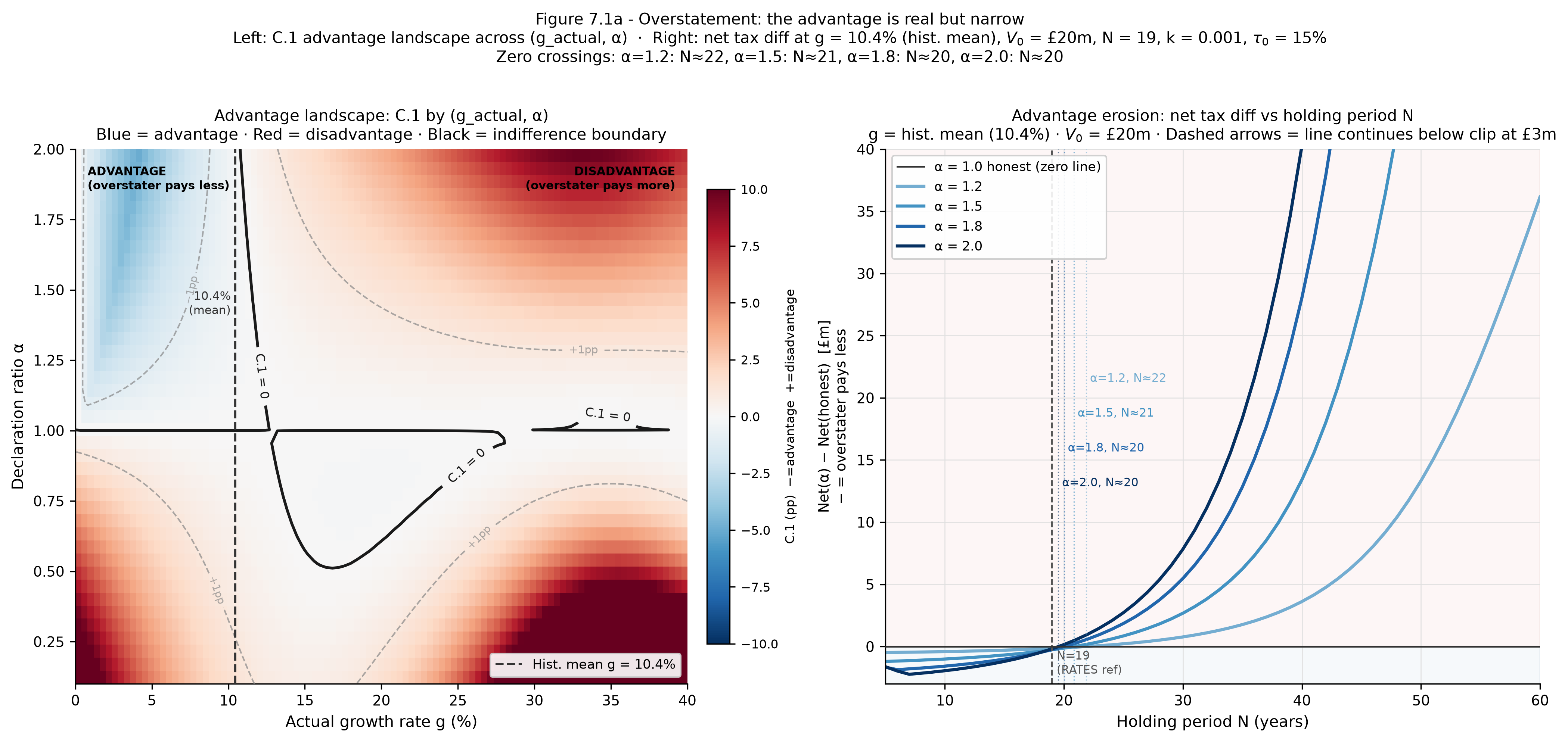
The C.1 scale in the left panel captures structural incentive shape as a percentage of terminal wealth; the right panel’s absolute £m scale captures practical magnitude at the canonical reference position. Both panels are needed for a complete reading: the left establishes which (\(g\), \(\alpha\)) combinations are net-costly, the right shows how the cost accumulates and crosses into net disadvantage as holding period extends.
Figure 7.1b extends the picture to the full declaration range at multiple growth rates, plotting net tax relative to honest as a continuous function of \(\alpha\). The 2000 start-year historical series (mean \(g\) \(\approx\) 6.0%, purple dash-dot) diverges materially from the constant-\(g\) lines at overstater \(\alpha\) values, reflecting the lower mean realised growth. The clustering of lines near zero in the \(\alpha\) = 0.8 to \(\alpha\) = 1.5 range at moderate constant growth rates is the tolerant zone made visible as a continuous curve rather than a heatmap region. The U-shape of the aggressive overstater lines confirms the growth-corridor structure: advantage at very low growth, a net-cost region above \(g\) \(\approx\) 7%, and partial recovery at very high growth.
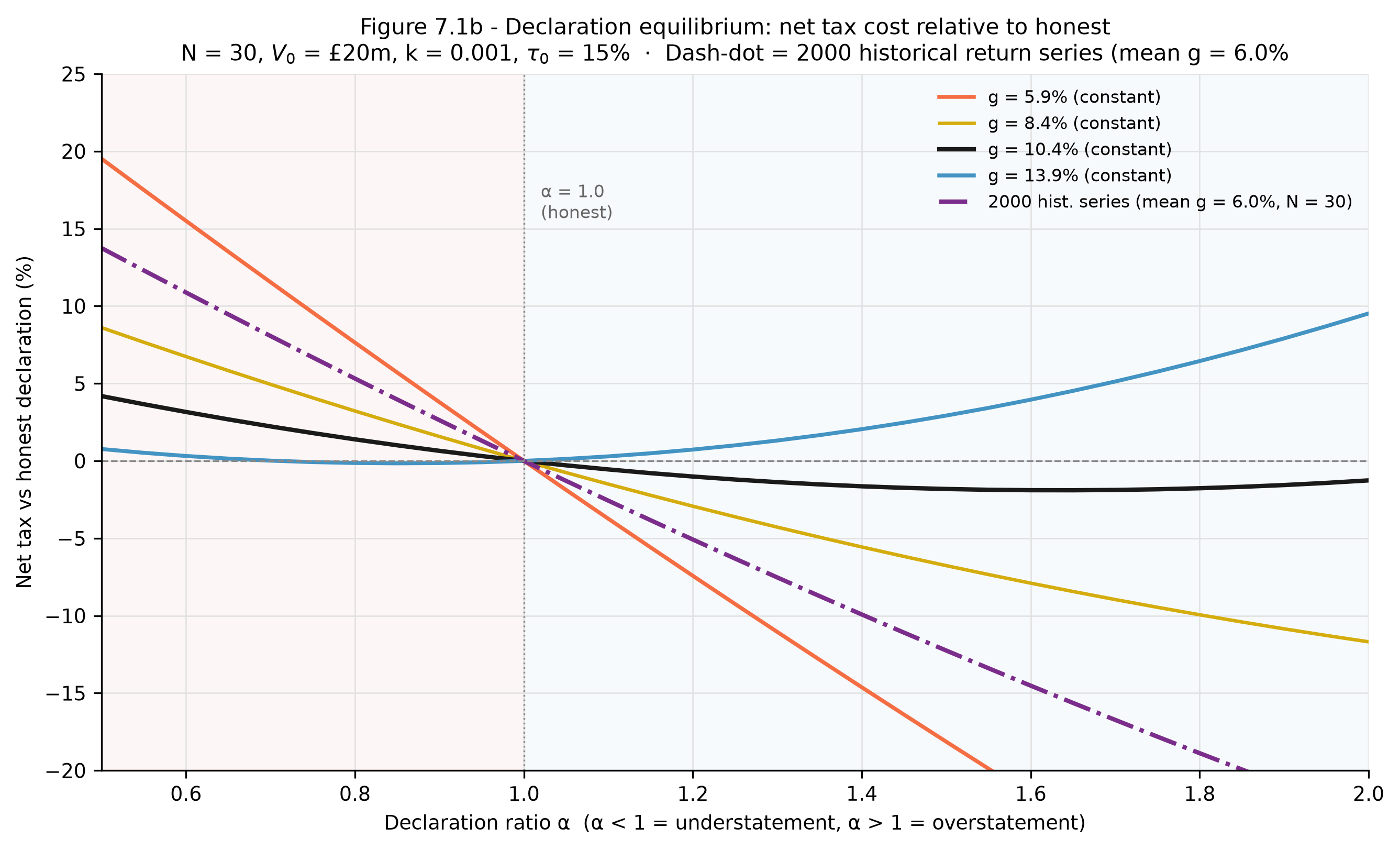
Figure 7.1c maps the nominal TW_settled advantage across the full (\(g\), N) surface for all four tested \(\alpha\) levels. Each panel shows that the nominal advantage is positive throughout — overstatement always retains more nominal TW_settled than honest declaration across the tested range — but these figures do not represent a genuine economic advantage once discounting is applied. For \(\alpha\) = 1.2, the nominal advantage peaks at 2.6pp at approximately \(g\) = 0.6%, N = 34; for \(\alpha\) = 1.5, at 6.5pp near \(g\) = 1.1%, N = 41. These peaks occur at low growth and long horizons precisely where the discounting penalty is greatest: a refund received at N = 41 is worth far less in present-value terms than the periodic outflows that precede it. At the canonical intersection (\(g\) = 10.4%, N = 30, red dot), the nominal advantage from (VAL.A §C.11) is approximately 2.4pp for \(\alpha\) = 1.2 and 6.0pp for \(\alpha\) = 1.5; both are reversed under NPV adjustment at ρ = 5% (VAL.A §C.12). Aggressive overstatement panels (\(\alpha\) = 1.8, 2.0) show the same nominal pattern but additionally face a contemporaneous growth-corridor cost, consistent with the N-crossing results in (VAL.A §A.5.4).
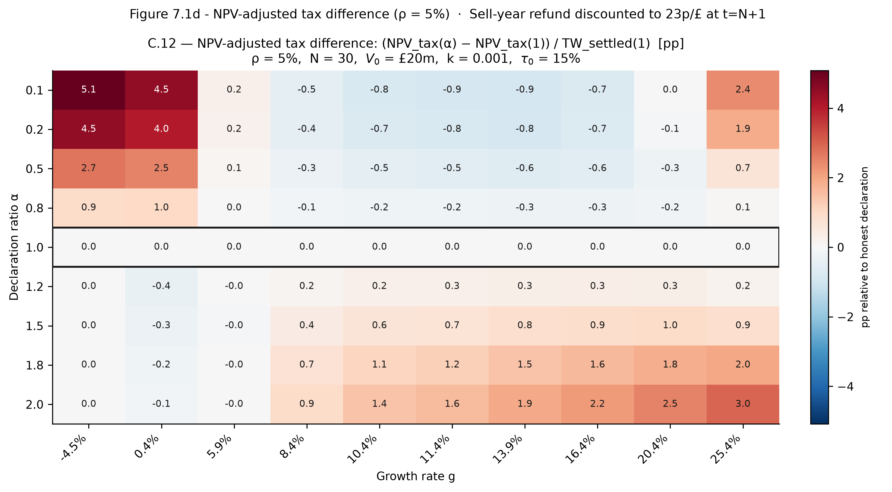
Periodic tax payments accumulate throughout the holding period at the rate the declared wealth commands in each year; the sell-year refund arrives as a single payment at year N+1. The nominal TW_settled advantage is therefore measured by comparing earlier outflows against a later inflow without adjusting for the time value of money. Figure 10 quantifies what happens when that adjustment is applied. At ρ = 5%, a cash flow at year 30 is worth approximately 23 pence on the pound relative to a year-1 payment. In the low-growth band (\(g\) ≲ 8%) — the only band where C.1 shows a nominal advantage for mild overstaters — the NPV-adjusted C.12 metric compresses that advantage sharply: from −0.91pp to −0.29pp for \(\alpha\) = 1.5 at \(g\) = 0.4%, and from −1.66pp to −0.04pp at \(g\) = 5.9%. The nominal advantage exists in those cells; the discounted advantage does not.
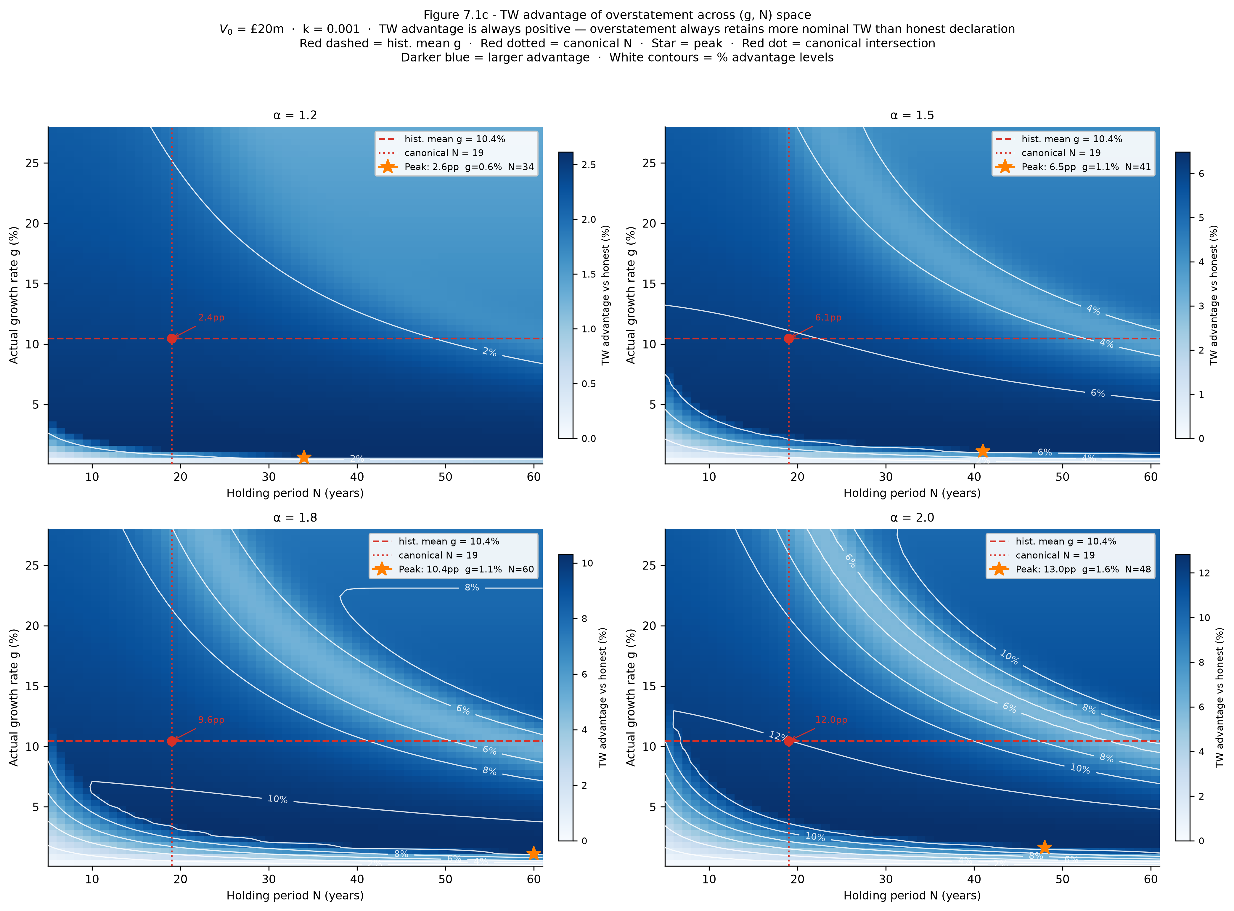
Figure 7.1d makes the two-regime structure visible directly. The left panel reproduces the C.1 nominal metric; the right panel shows C.12, the same metric discounted at ρ = 5%, on an identical colour scale. The compression of the low-g blue cells toward white or red in the right panel is the quantified answer to the caveat: the mild-overstater nominal advantage is a timing artefact that does not survive discounting. Understater penalty cells (red, upper rows) remain broadly stable across both panels, confirming that the excess cost of understatement is real in both nominal and present-value terms.
Simulation results across the tested strategies are in (VAL.A §C.1). The formal model supporting these claims is in (VAL.A §A), with the local convexity result at (VAL.A §A.5.1) (Proposition 1) and the full proposition summary at (VAL.A §A.5.6). Worked examples illustrating the payoff-profile argument are in (VAL.B §N).
7.2 Understatement: Deferred Liability and Dilution
Understatement changes the timing and form of taxation but does not generally eliminate the underlying claim. The declared value establishes the recognised basis from which future changes are measured. Where the asset appreciates, the gap between that basis and the eventual economic value grows, recovered through periodic delta assessment for fungible assets or the realisation event for non-fungible assets.
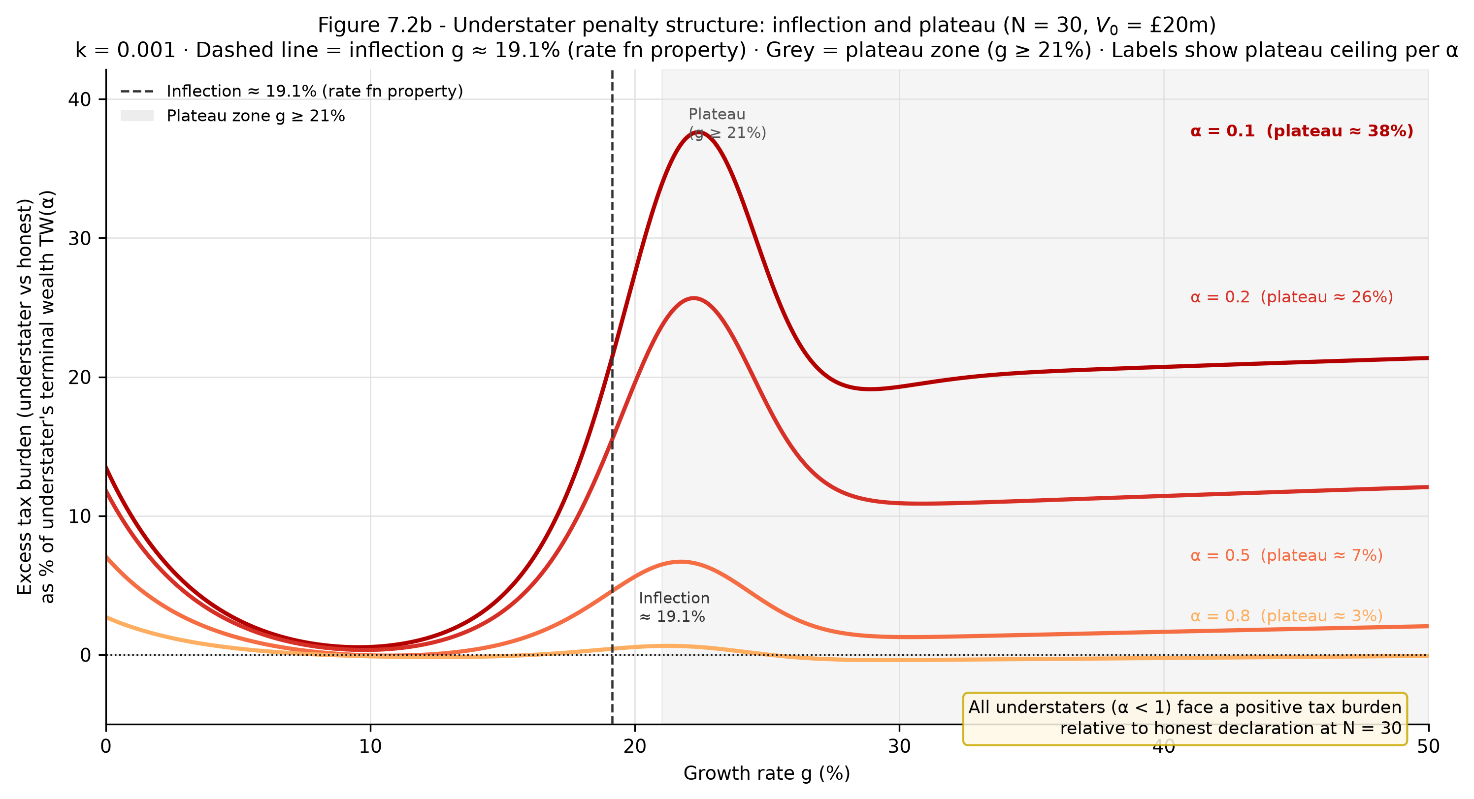
Across the policy-relevant growth range, the economic cost of understatement increases with asset growth rate and holding duration. The marginal deterrent escalates steeply between \(g\) \(\approx\) 10% and \(g\) \(\approx\) 19%, then plateaus: the rate ceiling stops further escalation but does not reverse the penalty. The plateau ceiling is proportional to the degree of understatement. The full profile across growth rates is in (VAL.A §C.9).
Figure 7.2a shows the TW_settled gap against holding period for both understaters and overstaters. The figure plots both constant-\(g\) lines (solid red for understaters, dashed blue for overstaters, at \(g\) = 10.45%) and the 2000 historical return series (dash-dot red and dotted blue respectively, mean \(g\) \(\approx\) 6.0%). Understater penalties widen substantially as N increases under both series; overstater TW_settled advantages are broadly stable. Mild understaters (\(\alpha\) = 0.8) show modest and relatively stable penalties throughout; severe understaters (\(\alpha\) = 0.1, 0.2) show dramatic penalties at long N under the constant-\(g\) series, with the historical series producing qualitatively similar but compressed results. The cost asymmetry is a time-compounding effect, not merely a growth-rate one.
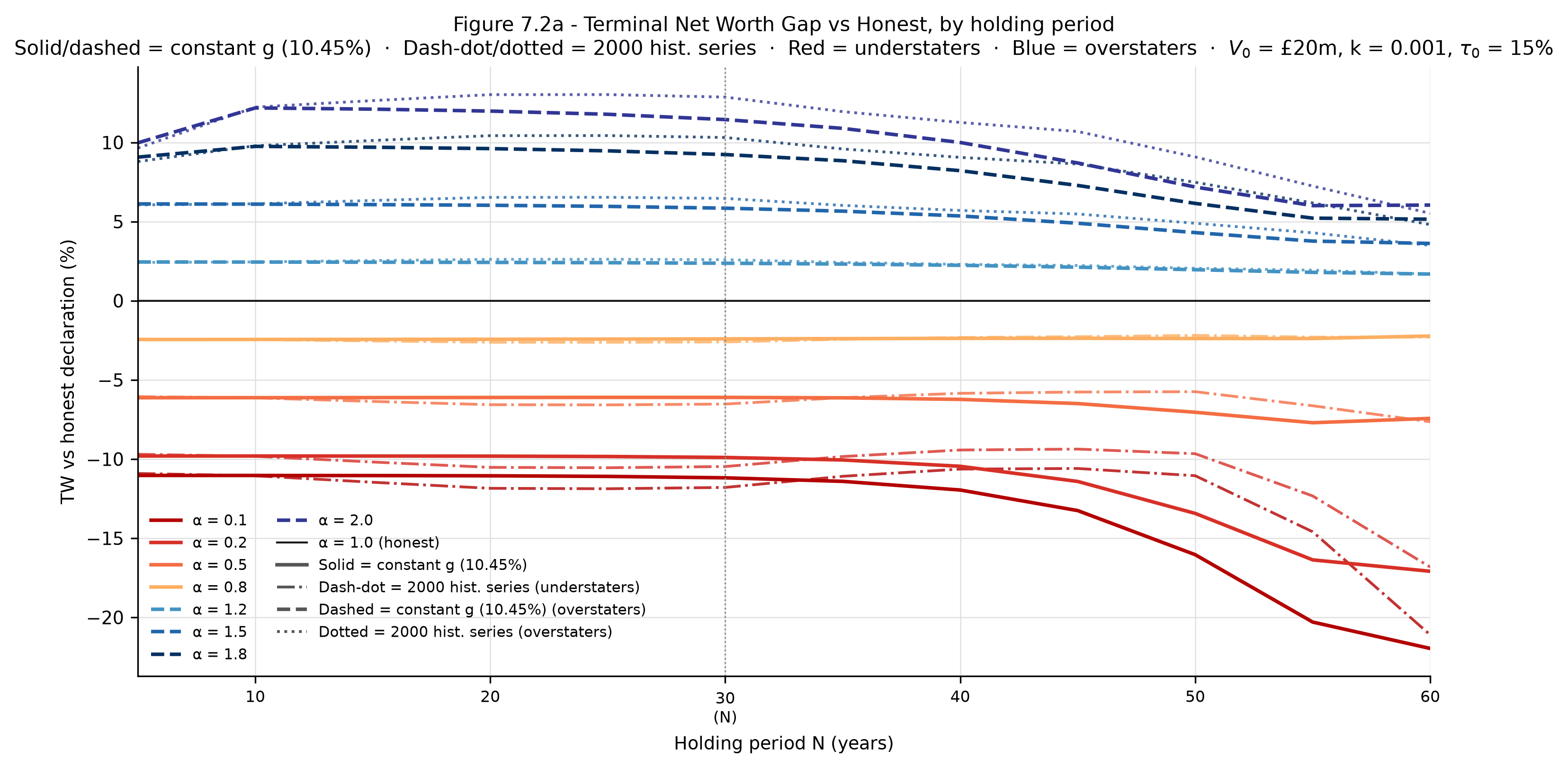
Figure 7.2b shows the plateau structure directly. The excess tax burden for each understater strategy rises steeply through the \(g\) = 10–19% range, then flattens at a ceiling proportional to the degree of understatement: approximately 38% of terminal wealth for \(\alpha\) = 0.1, 26% for \(\alpha\) = 0.2, 7% for \(\alpha\) = 0.5, and 3% for \(\alpha\) = 0.8. The penalty does not reverse above the plateau; the rate function simply stops escalating. The inflection value visible in the figure is approximately \(g\) \(\approx\) 19.1% at N = 30; (VAL.A §C.9) and (SWEEPS §2.3) establish this as a rate-function property that is approximately constant across all \(\alpha\) and N-invariant above the plateau.
For fungible assets, the must-transfer mechanism creates an additional direct cost through equity dilution. The stronger the asset performs, the larger this implicit cost becomes, which is why the deterrence is strongest for the largest, fastest-growing positions.
The incentive is state-contingent. For rapidly appreciating assets, understatement is generally unattractive because deferred liability and dilution effects compound with growth. For assets that subsequently fail, understatement can produce a measurable benefit: the taxpayer avoided paying tax on wealth that did not ultimately exist. The WDT accepts this outcome as an unavoidable consequence of taxing uncertain future wealth rather than retrospectively reconstructing historical values. Worked examples are in (VAL.B §J) and (VAL.B §K).
7.3 Overstatement: Signalling and Confidence Effects
Overstatement increases the immediate WDT liability through a higher marginal rate position, but valuations also perform an economic signalling function. A higher declared value may influence investors, lenders, counterparties, and employees in ways that create real economic benefits external to the tax system. The WDT places a price on this behaviour rather than eliminating it: a taxpayer who declares a higher value receives any associated signalling benefit but accepts the corresponding fiscal consequences.
The outcome depends substantially on degree. On a nominal TW_settled basis, declarations within the overstatement side of the tolerant zone (\(\alpha\) ≤ 1.5 at canonical parameters) retain more terminal wealth than honest declaration at low growth — the inflated basis generates a sell-year refund that nominally exceeds the f_N erosion and post-sale damping costs (VAL.A §C.11). However, this nominal advantage does not represent a genuine economic return: (VAL.A §C.12) shows that once all cash flows are discounted at ρ = 5%, the advantage collapses or reverses throughout the growth range where it nominally exists. Moreover, even the nominal advantage is conditional: C.1 turns positive (the mild overstater pays more than honest declaration) above approximately \(g\) \(\approx\) 7% for all tested \(\alpha\) levels at N = 30. Since the historical mean growth rate is 10.4%, mild overstatement is in nominal net-cost territory at the historical mean. The overstatement side of the tolerant zone is better described as: declarations that produce small lifetime tax differences from honest declaration at low to moderate growth, but without a meaningful economic return at any growth rate once discounting is applied.
The specific illustrative values (\(\alpha\) = 1.2 retains approximately +2.4pp nominal TW_settled advantage at the canonical intersection; \(\alpha\) = 1.5 approximately +6.0pp) are representative points on the overstatement side of the tolerant zone, not evidence for a wealth-maximising equilibrium. They describe a nominal timing artefact, not an economic return.
Aggressive overstatement (\(\alpha\) ≥ 1.8) exits the tolerant zone and faces an additional contemporaneous cost. The bracket penalty is large enough to produce a net cost relative to honest declaration throughout the \(g\) \(\approx\) 9–17% corridor — the range containing the historical mean and the majority of realistic trajectories. The aggressive overstater’s net advantage nominally recovers only outside that corridor, and even there it is bounded and eliminated by NPV adjustment. The quantitative bounds are in (VAL.A §C.1), (VAL.A §C.12), and (VAL.A §A.6).
The genuine rationale for a mild upward declaration bias is asymmetric refund protection under valuation uncertainty. A taxpayer who does not know the precise value of their asset faces a declaration problem with a natural error band — typically ±10–20% for illiquid private assets. The cost function around honest declaration is not symmetric in the refund dimension: an understater who is wrong in a bad year receives a materially smaller refund (VAL.A §C.6); an overstater in the same bad year receives a larger one. A risk-averse taxpayer aware of this asymmetry would rationally centre their declaration slightly above their central estimate — at approximately \(\alpha\) \(\approx\) 1.1 rather than \(\alpha\) = 1.0 — so that the negative end of their uncertainty band still lands in overstatement territory, preserving a larger refund entitlement in a loss year. This is a conditional behavioural prediction contingent on the assumed uncertainty and risk preferences, not an equilibrium in the sense of a dominant strategy.
Overstatement is therefore not a failure mode the mechanism needs to prohibit — it is self-regulating within the tolerant zone and self-limiting beyond it.
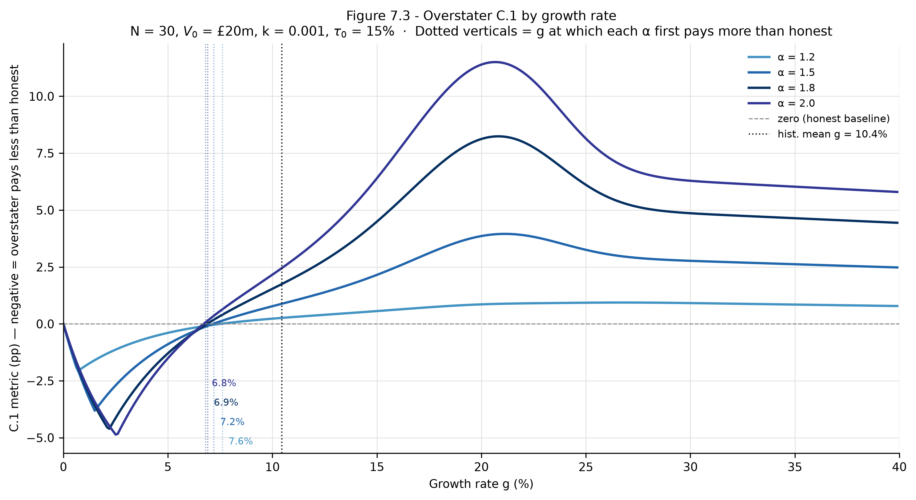
Figure 7.3 shows the C.1 net-tax structure directly. The panel plots C.1 by growth rate for four overstatement levels. All four lines begin negative at low \(g\) — mild overstaters pay less net tax in nominal terms throughout the low-growth range. Each line then crosses zero at a first-reversal threshold (annotated as approximately 6.8% for \(\alpha\) = 2.0 through 7.6% for \(\alpha\) = 1.2), confirming that even mild overstatement is in net-cost territory above those thresholds at N = 30. \(\alpha\) = 1.8 and \(\alpha\) = 2.0 show a secondary partial recovery above \(g\) \(\approx\) 20%. The historical mean \(g\) = 10.4% (dotted vertical) sits above all first-reversal thresholds, placing all four strategies in net-cost territory at the historical mean. C.1 < 0 for mild overstaters at low \(g\) reflects the nominal metric only; as (VAL.A §C.12) establishes, the NPV-adjusted version is near-zero or positive once discounting is applied.
A key asymmetry: in negative growth scenarios, understaters do not recover the same refund as honest declarers. The refund is proportional to the declared basis, not the true value, so an understater who declared at a fraction of true value recovers a materially smaller refund. The precise reduction at RATES-aligned parameters is in (VAL.A §C.6). The TW shortfall in loss years flows from the refund shortfall, not from any additional tax liability.
7.4 Boundary Conditions and Limitations
If a taxpayer understates a company that subsequently fails completely, the understatement produced a real benefit: less tax was paid on wealth that turned out not to be durable. The WDT accepts this. A system that tries to reconstruct accurate valuations retrospectively for failed assets is pursuing a fiction.
There is a partial counterweight: an understater receives a smaller refund on failure because the refund is calculated on the declared basis rather than the true value. At RATES-aligned parameters, the reduction is directionally large rather than marginal: at \(\alpha\) = 0.5 the understater retains 93.78% of the honest declarer’s TW_settled in a loss year; at \(\alpha\) = 0.1, 88.30%. A taxpayer who systematically understates loses meaningful protection in bad years, which reinforces the incentive to declare honestly. Full results are in (VAL.A §C.6).
A related design choice affects all loss years. The refund rate is \(\tau(W_t)\) — the rate implied by current declared net worth — not the rate that applied in the gain year. A taxpayer falling from £500m to £200m receives a refund at the £200m rate. The state captures gains at a higher marginal rate than it shares equivalent losses when net worth has moved between brackets. The alternative — applying \(W_{t-1}\) — would give taxpayers an incentive to overstate declarations before anticipated loss years to secure a higher refund rate, which is a worse exploit than the asymmetry it corrects. Full rationale is in (VAL.A §A.3.2).
See (VAL.B §J), (VAL.B §L), and (VAL.B §M) for the failure case and Route D entry basis vulnerability respectively.
7.5 Portfolio Composition as a Structural Constraint on Declaration Deviation
If the tolerant zone runs from \(\alpha\) = 0.8 to \(\alpha\) = 1.5 with relatively modest consequences within it, what prevents a sophisticated taxpayer from systematically anchoring at the lower edge? The answer is a constraint the simulation tables do not make explicit: \(\alpha\) is a portfolio-level aggregate, and for the population the WDT primarily addresses, a large share of that portfolio is structurally locked to \(\alpha\) = 1 regardless of declaration intent.
Routes A and B subject assets to independent professional valuation. The declared value is the valuator’s determination, not the taxpayer’s, which the mechanism treats as the operative basis. A taxpayer cannot self-declare a listed equity or a professionally appraised property at a fraction of its independently established value without triggering inconsistency immediately detectable by the Administrator. Route A and B assets carry an imposed \(\alpha\) = 1 and contribute no leverage to a declaration strategy directed at the portfolio aggregate.
Portfolio \(\alpha\) is a weighted average. A taxpayer with proportion p of their wealth on Routes A or B and proportion (1 − p) on Routes C or D has:
\(\alpha_{portfolio} = p · 1 + (1 − p) · \alpha_{C/D}\)
where \(\alpha\)_C/D is the declaration ratio applied to their self-declared assets. To achieve a target portfolio \(\alpha\), the required C/D declaration ratio is:
\(\alpha_{C/D} = (\alpha_{target} − p) / (1 − p)\)
The structural anchor amplifies rather than merely limits deviation. A taxpayer with 60% of wealth on Routes A/B who wants a portfolio \(\alpha\) of 0.8 must declare their C/D assets at \(\alpha\) = 0.5; to reach \(\alpha\) = 1.5 they need $_{C/D} = 2.25. Extreme portfolio positions require increasingly implausible asset-level declarations.
The following table gives the required C/D declaration ratio across A/B share levels and target portfolio \(\alpha\) values:
| A/B share | Target \(\alpha\) = 0.7 | Target \(\alpha\) = 0.8 | Target \(\alpha\) = 1.2 | Target \(\alpha\) = 1.5 |
|---|---|---|---|---|
| 30% | 0.57 | 0.71 | 1.29 | 1.71 |
| 50% | 0.40 | 0.60 | 1.40 | 2.00 |
| 60% | 0.25 | 0.50 | 1.50 | 2.25 |
| 75% | 0.00 | 0.20 | 1.60 | 2.50 (impossible if C/D assets are honestly worth less) |
| 80% | — | 0.00 | 1.50 | 2.50 |
A taxpayer at the 80% A/B level cannot achieve a portfolio \(\alpha\) below 0.8 without declaring C/D assets at values approaching zero (a declaration that triggers the Route D auction’s corrective pathway or, for Route C assets, an implausible must-transfer price the mechanism enforces directly). At the upper tail, the C/D declaration required for portfolio \(\alpha\) = 1.5 at 60% A/B exposure is 2.25, more than double the asset’s true value, and faces the full set of aggressive overstatement penalties analysed in §7.3 and (SWEEPS §2.2).
The constraint is strongest where the fiscal stakes are highest. (BEHAV.A §A.2) to (BEHAV.A §A.5) places Route A assets (listed equities, liquid financial instruments, pension wealth) at approximately 40–55% of total WDT-taxable wealth at the population level, concentrated disproportionately at the top of the distribution. The ultra-high-net-worth population with V₀ above £100m (the bracket (SWEEPS Figure 11c) shows generates the sharpest incentive landscape) also carries the highest structural A/B exposure. The taxpayers for whom revenue implications are highest face the tightest constraint on portfolio \(\alpha\) deviation from 1.0.
This does not eliminate declaration risk. Route D assets (privately held non-fungible positions) retain flexibility at entry, and the inception basis vulnerability noted in §14.4 applies with full force. The vulnerability is concentrated in the C/D fraction, not distributed across the whole portfolio. A taxpayer whose wealth is 70% professionally valued has 30% of their net worth available for declaration strategy; a 12% shortfall on that 30% is a 3.6% shortfall on the total, within the tolerant zone’s ±2% outcome range and bounded by the costs §7.2 and §7.3 establish on both sides of honest declaration.
Enforcement implications concentrate on a specific, identifiable place: C/D assets, particularly Route D, particularly at entry. The priority is the distribution of entry declarations at inception and at inheritance (the two moments where Route D basis is most exposed) and the pattern of declared values relative to realisation prices as Phase One data accumulates. That measurement agenda is specified in (PHASE1 §5.4), which should be read alongside this section.
9. The Public Valuation Register
Wealthy individuals can, in the absence of any consistency mechanism, maintain different valuations for the same assets across different legal and commercial contexts. The WDT addresses this through a publicly accessible register of declarations.
At each annual submission, taxpayers tag each asset as disclosed or private. Disclosed assets attract a rate discount from the standard marginal rate; private assets attract a rate premium. Only the disclosed portion flows into the public register. The privacy election is a choice between two equivalent forms of participation: disclosed taxpayers provide democratic visibility of the wealth base at personal cost through disclosure, while private taxpayers contribute financially through the premium. Full privacy for any individual taxpayer is compatible with the mechanism functioning identically in every dimension that matters — revenue is correctly calculated, refund symmetry operates, and the Route D auction deterrent rests on the committed declared value rather than on public register visibility. The operational specification of the privacy election, including the rate differential coefficient, the whole-asset requirement for non-fungible positions, and the personal security exemption, is in (GOV.B §B.4.7).
WDT declarations for disclosed assets are recorded in the register. Lenders, insurers, counterparties, courts, and potential buyers can see what a taxpayer has declared for WDT including the history of those declarations over time. When a taxpayer maintains a very different figure for the same asset in a different context, that inconsistency is visible to anyone who looks. Courts, insolvency practitioners, lenders, and counterparties may consider WDT declarations as one input among others.
The register does not bind courts to treat WDT valuations as correct in other proceedings. Those proceedings have their own valuation standards and purposes. The framework expects the register to raise the cost of maintaining inconsistent valuations across contexts by making those inconsistencies visible. Whether it does so in practice depends on how widely the register is consulted and whether courts and counterparties treat WDT declarations as meaningful reference points.
The register also allows taxpayers some visibility into each other’s declared values, enabling a degree of peer monitoring that does not depend on state capacity alone. The three-tier structure governing what the register makes public is specified in (GOV.B §B.4.6) and (GOV.B §B.4.7): governance outputs are fully public at tier one; declared asset values for disclosed assets are public at the figure level using stable reference IDs rather than personal identifiers at tier two; individual delta calculations, refund amounts, and lifetime envelope balances carry ordinary tax-record protection at tier three. The jurisdiction-specific data-protection law governing the reference-ID lookup mechanism is Phase One and (JUR) work.
One consequence of the mild upward declaration bias predicted in (VAL.A §A.6) — driven by refund-protection asymmetry under valuation uncertainty rather than by any genuine TW return to overstatement — is that the declared values in the register are likely to be systematically inflated relative to true asset values for the disclosed portion. A declared £12m on an asset worth £10m generates a correct negative delta and refund when it eventually sells, but the register entry is inflated throughout the holding period. Lenders and counterparties using the register as a reference point work from figures above true values — a credit-expansion effect on private asset-backed lending that is probably modest but real. Periodic hard price discovery at inheritance and Route D auction events anchors the register back to market values. The Administrator holds no instrument for signalling systematic drift in the population distribution of declared values relative to true values; Phase One data on declared values relative to subsequent realisation prices is the primary detection mechanism.
Two categories of third-party use warrant explicit disclaimer. First, credit decisions: declared values reflect a taxpayer’s assessment-date commitment for delta-calculation purposes and carry no state warranty as to market value. A credit officer treating a register entry as equivalent to a market appraisal is making an error the state has explicitly tolerated within its own design. Declared values may inform credit decisions as one weight among others; they may not serve as the sole or primary basis. Second, legal proceedings: the register was not designed as a valuation instrument for matrimonial, probate, or shareholder dispute purposes. The declared value is relevant evidence of a commitment made under penalty, not an independent appraisal of market value. Both disclaimers should appear on the face of the public register and in the Administrator’s mandatory publication cycle.
10. Professional Valuation
10.1 Purpose
The professional route exists for assets where methodology is established and independent assessment adds meaningful information at reasonable cost. It is not appropriate where the methodology range is too wide for certification to add value, or where assessment cost exceeds the revenue differential.
10.2 Competitive Tender Model
When a taxpayer elects professional valuation for an asset, they initiate an open tender among accredited valuation firms. The lowest qualified bid is selected, subject to independence requirements and conflict-of-interest screening.
Competitive tender rather than client appointment is a structural choice. The Pereira Gray (2021) identified the appointing relationship itself as a primary driver of valuation drift: a valuator who depends on referral and repeat engagement from a wealthy client develops institutional pressures toward lower values that no amount of professional accountability can fully counteract. A valuator who wins business through transparent price competition has a materially different relationship to the client.
For very large, concentrated, operationally complex private company positions, the number of qualified firms may be small. For this asset category, the independent review process carries more of the deterrence weight than the tender itself. Assets of this character tend naturally toward self-declaration.
10.3 Cost Sharing with a Fee Cap
The agreed valuation fee is split between the Taxpayer and the State on approximately equal terms up to a defined cap. Above the cap, the Taxpayer bears the full marginal cost.
Below the cap, the shared structure gives the State a financial stake in the first-stage assessment being defensible: a challenged assessment triggers independent review at Authority cost, creating an institutional incentive to monitor quality. Above the cap, increasing cost pressure makes the professional route progressively less attractive relative to self-declaration for complex assets.
10.4 The Two-Stage Review Process
The selected valuator presents their determination to the Taxpayer. On acceptance, the valuation is final for the assessment window, shared between the Taxpayer and the State. On rejection, the Taxpayer assumes responsibility for the State’s share of the original fee; the Authority uses those freed funds to commission an independent review, covering any excess.
Independent review produces one of three outcomes. If it supports the original valuator, the original valuation stands and the Taxpayer bears the full cost of the original fee. If it supports the Taxpayer, the Taxpayer’s position is accepted and the original valuator’s contract is terminated with no compensation. Where the review supports neither party, the asset transitions to the applicable self-declaration route for that assessment cycle: Route C for fungible assets, Route D for non-fungible assets.
10.5 The Valuation Code
The Valuation Code governs the professional route. It specifies asset-class-specific methodology hierarchies, parameter ranges within which professional judgment may legitimately operate, disclosure requirements for methodology selection, and procedural standards for WDT-accredited work.
The Code’s starting point is the IVSC observable-to-unobservable methodology hierarchy, which establishes a preference for directly observable market inputs and requires disclosure of methodology where unobservable inputs are used. One important distinction from financial audit practice: IFRS 13 and ASC 820 frame audit opinion as expressing a range of acceptable values. The WDT requires a single assessed value for tax calculation. The profession must adapt accordingly.
The most directly applicable governance precedent is the Pereira Gray (2021). The Valuation Code should build on that framework, extending it on three dimensions: the elective assessment cadence rather than transaction-triggered valuation; cross-context public consistency through the register; and incentive alignment at the top of the asset complexity range where the Pereira Gray reforms remain weakest.
For standard residential property, automated valuation models calibrated to comparable sales and land registry records can handle routine assessment. Where a model diverges materially from the prior window’s certified value, professional valuation is triggered.
10.6 Valuation Governance
The Valuation Code Board is an independent statutory body responsible for maintaining and amending the Valuation Code. It is not part of the tax authority and is not under ministerial direction. Its statutory mandate cannot be changed except through primary legislation.
Without governance, methodology drifts toward lower valuations over time, a pattern well-documented in professional valuation contexts where the regulated population has better information and stronger incentives than the regulator (Pereira Gray, 2021). The Board includes representation from the valuation profession, government, academic economists, and public interest observers. No single constituency holds a majority. Profession representation is necessary; profession-majority governance is not.
Public interest representation requires institutional support. (GOV §6) (DR mandatory voting and seat-burn mechanics) and (GOV.A §A.1) (constituency dissolution mechanism) address the Olson problem facing multi-constituency bodies of this kind; the DR chamber’s lottery-selection model and monthly staggered turnover are the mechanism GOV adopts against that dynamic, and they provide the relevant design precedent for how the Valuation Code Board’s public interest block should be organised. The Valuation Code Board is a separate entity from the Valuation Bodies outlined in (GOV §6.1); the Board publishes best practices for the professional valuation industry, while the Bodies are WDT Executive bodies responsible for audit, valuation disputes as outlined in (VAL §10.4) and investigating Route D outliers.
11. The Route D Auction Mechanism — Three Uses of One Process
The Route D auction fires in three distinct circumstances, each with its own initiation architecture and tax treatment.
Corrective auction (VAL §11.3): triggered when two independent Valuation Bodies, working without knowledge of each other’s findings, corroborate a flag raised by a third that the declared value is an egregious statistical outlier. The taxpayer does not initiate. The mechanism operates against both under-declaration and over-declaration.
Voluntary hard-reset auction (VAL §11.2): requested by the taxpayer to obtain a market-tested basis before a forced realisation event. No Valuation Body involvement required. The purpose is certainty for the taxpayer, not enforcement.
Inheritance auction (VAL §11.4): triggered automatically when a Route D asset passes to an heir. No taxpayer election and no Valuation Body consensus required; the transfer event is the trigger.
All three share the same auction mechanics: the asset is offered at the most recent recognised declared value as the opening price, any willing buyer may bid, and the winning bid becomes the new recognised basis. What differs is who triggers the process and what tax treatment follows.
11.1 Deterrent Logic
The corrective auction is the deterrent of last resort for egregious misdeclaration of self-declared non-fungible assets. Routes A and B are professionally valued; mispricing liability rests with the valuator. Route C’s must-transfer rule creates continuous self-correction through dilution. Route D has no analogous interim correction: between entry declaration and realisation, a misdeclared basis compounds forward without automatic adjustment. The corrective auction closes this gap where Valuation Body consensus confirms it exists.
The logic draws on the Harberger self-assessment tradition (Harberger (1965)). A taxpayer declaring a private estate at £5 million when it is worth £80 million faces losing it at the price they asserted was fair. The cost of the misstatement falls on the person who made it. The state never needs to assert a correct value; the market supplies it.
11.2 Voluntary Hard-Reset Auction
A taxpayer may request an auction at any time during the holding period to replace an uncertain self-declared basis with a market-tested value. The taxpayer applies directly through the Administrator; no Valuation Body involvement is required.
Where the auction establishes a value above the prior declared basis, the taxpayer may sell at that price or retain the asset with the auction price as the new recognised basis, paying WDT on the upward delta in the normal way.
Where the auction establishes a value below the prior declared basis, the taxpayer may sell or retain. On retention, the auction price becomes the new recognised basis and the downward delta generates a refund entitlement under the symmetric mechanism, subject to the lifetime contribution envelope. The voluntary hard reset does not carry the corrective no-refund rule.
Auction costs are borne by the taxpayer.
11.3 Corrective Auction: Trigger and Process
The corrective trigger is strict. A Valuation Body finding a Route D declared value to be a statistical outlier raises a flag and is excluded from what follows. The Administrator assigns the asset independently and simultaneously to the other two Valuation Bodies, without disclosing that a flag has been raised or what gap ratio triggered it. Each body produces a sealed independent estimate. The Administrator opens both estimates simultaneously. If both non-flagging bodies find, independently, that the gap between the declared value and their own estimate exceeds the trigger threshold, the Administrator publishes an auction notice. If either body fails to corroborate, the flag lapses without consequence to the taxpayer.
The taxpayer is not notified when a flag is raised or during the estimation period. Notification occurs only when the Administrator publishes the auction notice following confirmed corroboration. Notifying at the flag stage would allow a taxpayer to race to a soft basis reset before sealed estimates are submitted, defeating the mechanism. Once both non-flagging bodies have submitted their sealed estimates, the position is locked; no subsequent soft or hard reset affects the basis for that cycle.
The full three-body protocol, sealed-estimate sequencing, and non-anchoring requirement are specified in (GOV.B §G).
Under-declaration (P > B): The auction price exceeds the declared basis. The taxpayer may sell at the auction price, or retain the asset with the auction price as the new recognised basis and pay WDT on the upward delta. The gap between the original declared value and the auction price is a large positive delta in the auction year, taxed at the applicable marginal rate. Administrative fees are charged to the taxpayer.
Over-declaration (P < B): The auction price falls below the declared basis. The taxpayer may sell or retain. On retention, the auction price becomes the new recognised basis. No refund is generated by the downward correction. Historical WDT paid under the prior declared basis is not retrospectively recalculated. The reduction is a correction of an erroneous basis, not a realised loss; the corrective no-refund rule prevents a taxpayer from manufacturing refund entitlements through deliberate inflation followed by market correction.
No-bid outcome: Where the auction produces no valid bid, the asset is worthless. A public auction that attracts no bid is price discovery; the basis resets to zero in both directions. No professional valuation fallback is introduced: a professional estimate of what a willing buyer might pay cannot improve on the revealed answer that no willing buyer exists at any price. The no-refund rule applies on corrective over-declaration; on corrective under-declaration, a zero-basis reset generates no delta relative to a declared value that was already effectively zero, and ordinary mechanics apply from that point.
11.4 Inheritance Auction
When a Route D asset passes to an heir, the inheritance auction fires automatically. The asset is offered at the most recent recognised declared value as the opening price, any willing buyer may bid, and the estate holds the right to retain at the highest third-party bid price.
The inheritance auction is not a corrective event. The symmetric refund mechanism applies in full: where the auction establishes a value below the prior declared basis, the estate receives a refund entitlement on the downward delta, subject to the lifetime contribution envelope. The heir’s WDT entry basis is the auction price regardless of outcome.
Where the auction attracts no meaningful bids, the asset has no market value. Assets of negligible market value carry negligible WDT liability. Where an asset carries a significant prior declared basis but attracts no bids, the symmetric refund logic addresses the loss. A minimum professional valuation may be required as a fallback where no observable market exists and the basis requires establishing for succession purposes; this is assigned to (JUR §4.2).
The architecture governing auction conduct, timeline, estate retention rights, and no-bid fallback is in (GOV.B §G).
11.5 Scope
Rarity is a structural feature of the corrective trigger specifically. A mechanism triggering routinely would shift the institutional relationship toward the adversarial and undermine the cooperative logic the WDT depends on. The deterrent rests on credibility, not frequency. The voluntary and inheritance pathways are different: the voluntary hard-reset is available on demand and expected to be used regularly by taxpayers seeking a verified basis before death, a financing event, or a dispute; the inheritance auction fires automatically at every generational transfer of a Route D asset.
Inheritance is the point at which the voluntary option becomes compulsory. The process is identical; the trigger differs.
12. Administration and Fraud Detection
The professional valuation architecture in (VAL §10) is described in some detail because the design choices there — competitive tender, financial consequences for overturned valuators, the two-stage review — are not obvious extensions of existing practice and require explanation. The administration and fraud detection material that follows is comparatively brief. The delta structure’s self-correcting properties concentrate real risk on the parties making declarations, which shifts the Authority’s attention away from valuation disputes and toward fraud.
12.1 Annual Reporting Requirements
Taxpayers file an annual return to the Administrator regardless of assessment window selected. The full specification of reporting requirements is in (VAL.A §F). Third-party reporting obligations apply to financial institutions, listed company registrars, and land registries; their reports are distributed to the Valuation Bodies and used to cross-check returns. The interaction between individual-level reporting and the corporate withholding model for listed shareholdings is addressed in (CORP).
12.2 The Purpose of Audit: Fraud, Not Valuation
Once the self-correcting properties of the delta structure are understood, the Valuation Bodies’ enforcement role narrows considerably. (VAL.A §A.5.1) (Proposition 1) and (VAL.A §A.5.2) (Proposition 2) establish formally that deviations from honest declaration generate increasing costs through either dilution effects or rate effects. Most enforcement effort is therefore better directed at fraud than at valuation disputes; attempting to adjudicate whether a private company is worth £80 million or £100 million at scale would consume resources without proportionate benefit.
The Bodies’ primary enforcement function is identifying behaviour that prevents the delta mechanism from operating at all: hidden assets that never enter any declared net worth figure, fabricated transactions designed to manipulate recognised basis, sham ownership structures that conceal beneficial ownership, and criminal concealment of wealth through offshore or nominee arrangements. These are fraud investigations, not valuation disputes.
12.3 Statistical Review
The Valuation Bodies maintain a database of declared values, delta patterns, deferred balance positions, and third-party data. Declarations that are statistically inconsistent with comparable portfolios are flagged for inquiry.
The purpose of statistical review is not to find taxpayers who have declared slightly below market value. It is to find patterns suggesting that assets are not in the declared net worth figure at all, or that transactions have been structured to generate false basis adjustments. Statistical outlier detection operates in both directions: a declaration pattern persistently above all observable evidence of actual value, where this appears designed to generate refund entitlements, is a form of fraud rather than valuation disagreement.
12.4 Penalties
Penalties should not punish valuation disagreement. Honest differences of opinion about what an illiquid asset is worth are normal and expected. Two tiers are sufficient. Honest error and good-faith valuation disagreement attract correction to the revised value plus interest on the unpaid delta, with no additional penalty. Deliberate misstatement, evidenced by contemporaneous documentation inconsistent with the declared value, or participation in fabricated transactions, attracts a significant multiplier penalty and may be referred for criminal investigation where the scale warrants it.
13. The Sovereign Liquidity Facility
For taxpayers on any cash-settled route who face a WDT liability without ready liquidity, the Sovereign Wealth Fund may offer a credit facility secured against the declared or assessed asset value. Taxpayers may also pay directly, borrow privately, or liquidate assets. The tax design functions regardless of which financing route is chosen.
The facility is a Phase Two feature. It will come online incrementally as the SWF accumulates sufficient reserves and the operational infrastructure matures. Its purpose is partly political: it removes the objection that the WDT forces asset liquidation, and provides a state-backed option for taxpayers who cannot access private credit at reasonable terms against illiquid collateral.
The SWF holds three distinct credit instruments addressing different liquidity mismatches. The sovereign liquidity facility described here addresses the individual taxpayer’s annual liability without ready cash. The bridging facility (GOV.B §E.3) addresses a different mismatch: it decouples an individual’s physical departure from settlement of their personal WDT position at closure, operating through a bond structure rather than a secured lien. The corporate equity settlement facility (CORP §6) addresses the liquidity mismatch between a listed company’s assessment-date obligation and its cash generation cycle, through a secured lending arrangement under which the company transfers shares to the SWF in lieu of cash. All three are held in separate SWF portfolios with distinct mandate specifications.
Taxpayers may also elect to receive refunds in any portion of SWF units or cash. The governance rights attaching to SWF units are specified in (GOV.B §E.4): unit holders hold ordinary shareholder-type rights scoped to the fund’s own constitutional documents, including economic rights, information rights, and limited voting on major structural changes to the fund’s internal rules; they hold no Governing Council vote, seat, or standing.
Route C does not use the facility because that route settles in kind by definition. Where the facility is used, the state’s claim is structured as a secured lien against the asset.
14. Limitations and Further Work
14.1 Formal Modelling Gaps
No items in this paper. The tolerant zone result (\(\alpha\) \(\approx\) 0.8–1.5) and the route architecture developed here are used by (WFR §6.1.3) as the basis for Category 3 cost identification: valuation friction under Route D and the empirical compliance cost at scale are the two implementation costs WFR names as unquantifiable without Phase One data. VAL establishes the architecture from which those costs are derived; WFR establishes the welfare baseline against which their magnitude would need to be measured to determine whether they offset the Category 1 welfare costs of existing systems.
14.2 Phase One Empirical Unknowns
The Python model (v1.0) is validated with confirmed figures at unified parameters. Directional claims stand: understatement is more expensive than honest declaration across the policy-relevant growth range, and aggressive overstatement provides no reliable advantage at moderate growth. The model produces a broad tolerant zone spanning approximately \(\alpha\) = 0.8 to \(\alpha\) = 1.5 at canonical parameters, within which lifetime tax differences from honest declaration are economically negligible. Within that zone, consequences are asymmetric: understatement reduces refund protection in loss years while overstatement preserves it. This asymmetry gives risk-averse taxpayers under valuation uncertainty a modest incentive to bias their declaration upward, producing a model-implied behavioural centre near \(\alpha\) \(\approx\) 1.1. This prediction is conditional on the assumed uncertainty and risk preferences and is not an empirical estimate. The state’s objective is to collect the tax owed on actual wealth accumulation, not to enforce declaration precision. (VAL.A §C.1) confirms a wide region around honest declaration within which revenue collected is negligibly different from what exact honesty would produce; (SWEEPS) develops this point formally. Three empirical questions remain open.
First, whether the predicted mild upward declaration bias actually materialises, and at what magnitude, requires Phase One declaration data compared against independently assessed values on Routes A and B. Second, which assessment windows taxpayers actually elect, and in what distribution across routes, cannot be predicted in advance; Phase One election data is the primary input to any window-premium calibration. Third, the SRR floor calibration implication of any upward declaration bias (ENV §9.2) cannot be quantified before Phase One data establishes how far above \(\alpha\) = 1 the population centre sits.
The high-growth boundary condition (understater penalties plateau at approximately \(g\) \(\approx\) 19% at N = 30, and at \(g\) \(\approx\) 17.3% per the rate-function inflection established in (VAL.A §A.5.4) and (SWEEPS §2.3)) is a property of the bounded rate function, not a modelling error. The penalty does not reverse above the plateau; the marginal deterrent simply stops increasing. Directional claims hold across the policy-relevant growth range; Phase One route adoption and delta data will allow the Governing Council to assess whether any portion of the taxable population operates near that boundary.
Table C.3 in (VAL.A) carries deviations up to 13% at extreme \(\alpha\)×β values due to exponential compounding. Directional claims are unaffected. This is boundary behaviour at values outside the policy-relevant operating range.
14.3 Jurisdiction-Specific Legal and Implementation Work
The Route D entry basis is the mechanism’s named acceptable boundary condition. A low self-declared entry value establishes the basis from which future appreciation is calculated and is generally not independently verified; the Route D auction mechanism and public register provide deterrence only where assets have reliable comparables or where egregious understatement can be confirmed by three-body Valuation Body consensus. Where neither condition holds, the basis gap can persist.
Three things shape the boundary and limit its practical extent.
The conditions required to maintain the gap across a lifetime are mutually constraining. An asset generating WDT liability of meaningful scale at realisation will typically have produced at least one credible valuation signal during the holding period, through institutional financing, regulatory contact, employee equity, minority stake transactions, or litigation. The purest case of the residual — no external investors, no institutional credit, no valuation signals of any kind across a full holding life — is structurally rare. Real candidates fracture on this condition before realisation.
The gap is first-generation and self-diminishing. Subsequent generations inherit an auction-established basis, not a self-declared one. The comparables database that makes Route D audit more credible grows through ordinary operation. The entry basis vulnerability is concentrated in the WDT’s first cohort and narrows with time.
The extreme residual is an acceptable outcome on the WDT’s own terms. (MF §9.4.8) establishes this directly: the mechanism targets capital that exercises institutional and political power. A founder who never converts their position into that kind of power sits at the outer edge of what the design is trying to address, and accepting the extreme privacy case there is consistent with the foundational axiom. The basis gap in this case is a named consequence of correctly identifying the mechanism’s purpose.
What remains assigned to (JUR) is jurisdiction-specific: what supporting evidence the tax authority can require at entry declaration, and how disputes at that point are resolved through the relevant tribunal system. The policy trade-off is settled here.
The inheritance auction design-level questions are resolved: the mechanism uses auction price discovery, the heir chooses to retain or allow sale, and the auction price establishes the heir’s entry basis. Implementation questions remain open and are assigned to (JUR §4.2) and (JUR §4.3): auction conduct rules, the no-bid fallback procedure, timeline, and treatment of internationally-sited assets.
Cross-border holdings in jurisdictions outside existing information exchange frameworks remain a gap. International coordination and exit taxation design provide partial responses. Complete coverage is not achievable under current international arrangements.
One narrower derivatives question remains open: valuation methodology for derivative positions held for individual WDT purposes where no liquid secondary market exists. The double-counting risk is resolved by (CORP §8); this is a valuation question only, assigned to future methodology work.
14.4 Structural and Irreducible Limits of the Design
The mechanism has no clean exploitable holes, but it has boundaries. Three warrant explicit acknowledgment.
The inception basis boundary. The delta self-correction is powerful once an asset carries a committed prior value. The mechanism’s weakest moment is the first declaration: the grandfathering baseline at WDT launch, or the entry basis for a newly acquired Route D asset. At inception there is no prior value to self-correct against, and for Route D the external anchors available to Route A and B are absent. An understated entry basis does not eliminate liability; it defers and compounds it. But compounding runs silently across the holding period without the continuous correction Route C’s must-transfer mechanism provides. At realisation the final delta is calculated against the understated floor, hits a higher marginal rate bracket, and the taxpayer’s lifetime envelope refund entitlement is smaller than honest declaration would have produced. The Route D auction mechanism is the deterrent response; its effectiveness is bounded by how credibly it fires and how accurately competitive bidding reflects true value rather than auction-market dynamics.
The reclassification boundary. An asset transitioning from Route A or B to Route D through a legitimate structural change carries its prior committed value forward as the new Route D basis. Subsequent declarations accumulate delta against that basis without Route A and B’s self-correction mechanisms. Where reclassification is engineered to shift an asset from continuous market pricing to self-declared basis, the transition creates a window of reduced precision. The prior basis is correct at the moment of transition; subsequent drift from it is the residual this boundary admits.
The auction market maturation boundary. As the mechanism matures and professional participants develop expertise in the auction process, competitive behaviour may evolve beyond what the original design anticipated. Reset prices may come to reflect auction-market dynamics rather than underlying economic value, producing systematic overvaluation relative to private negotiated transactions. The hard reset was designed as a floor on understatement; in a mature auction market it may also function as a ceiling on privacy that sophisticated participants exploit in the other direction. This is an emergent property of the market the mechanism creates, not a design flaw, but it bounds the degree of control the auction process provides over final Route D valuation.
Phase One data on declared values relative to subsequent realisation prices is the primary detection mechanism. The measurement agenda in (PHASE1 §5.4) should treat the gap between entry basis and realisation price across the Route D population as a priority observable from the first assessment cycle.
Within-window asset composition management does not constitute a systematic exploit. Any conversion of a Route D asset — into cash, into another Route D asset, or into any instrument with a realisable value — triggers a realisation event at the point of conversion. The delta is calculated against the prior committed basis at that moment and captured in full. The lifetime envelope preserves contribution history across all conversion events. The assessment window accommodates flexibility in the timing of cash settlement; it does not permit the delta itself to be avoided through asset substitution.
14.5 Governing Council Calibration Parameters
The assessment window premium (deferral charge plus flexibility levy) is excluded from the RATES reference revenue model. Its calibration — the specific premium values for each window length — is a Governing Council parameter to be set once Phase One election data exists. The mechanism functions without it; its function is to price the deferral cost honestly rather than to generate revenue.
\(\tau_h\)’s calibration within [deterrence floor, \(\tau_m\)] for Route D purposes is a Governing Council parameter informed by Phase One attribution trend data. Addressed in full under (CORP) and (CORP.A).
15. Conclusion
The valuation problem for annual wealth taxation is real. Illiquid assets cannot be valued with precision every year, and no improvement in methodology can remove uncertainty where observable markets do not exist. But every prior proposal has framed the problem incorrectly. The question is not how the state determines the correct value of an asset the taxpayer prefers to undervalue. The question is whether the state needs to determine that value at all.
Under a conventional mark-to-market tax, it does: tax liability flows from true value, so the state must establish true value. Under the WDT’s self-declaration routes, it does not. The declared value becomes the legally operative basis. Tax liability flows from the delta between that basis and subsequent declared or realised values, calculated mechanically. The state’s task is to enforce the consequences of the declaration — not to certify whether the declaration was correct. Valuation accuracy ceases to be a necessary condition of tax administration.
This is not a modest reframing. It changes the category of problem the state is trying to solve. Enforcing declaration commitments, ownership records, and settlement obligations is a tractable administrative problem. Continuously adjudicating the correct value of every private company and illiquid asset at scale is not.
The WDT addresses this through a delta architecture. Professional routes place valuation responsibility with independent valuators while allowing flexible settlement. Self-declaration routes place responsibility with taxpayers and attach consequences to declared values. Under Route C, understatement creates a growing basis gap recovered through later assessment and an immediate dilution cost through the must-transfer rule; the declared price functions as a transaction price the taxpayer commits to stand behind, so the state acquires equity at whatever rate the taxpayer asserted was fair. Under Route D, periodic valuation is avoided by concentrating taxation at the point where an observable market value exists, eliminating the need for annual state certification of non-fungible asset values during the holding period.
The formal model and simulations in VAL.A provide supporting evidence that this architecture is not easily exploited. The primary finding is not that the mechanism forces accurate declarations — it does not — but that it creates a broad tolerant zone within which inaccurate declarations produce outcomes close to honest declaration, flanked by genuine penalties at the tails. (VAL.A §C.1) establishes that across declaration ratios from approximately \(\alpha\) = 0.8 to \(\alpha\) = 1.5, the lifetime net tax difference relative to honest declaration is economically negligible at the historical mean growth rate. Meaningful costs accumulate only at the tails: severe understatement at moderate-to-high growth, and aggressive overstatement at moderate growth. Within the tolerant zone, consequences are asymmetric: understatement reduces refund protection in loss years (VAL.A §C.6), while overstatement preserves it. This asymmetry produces a model-implied behavioural centre near \(\alpha\) \(\approx\) 1.1 under valuation uncertainty and risk aversion — a conditional prediction, not an empirical estimate. (VAL.A §C.11) decomposes the nominal TW_settled figures for the overstatement side of the tolerant zone: the sell-year refund benefit nominally exceeds the equity dilution and post-sale damping costs, explaining why the nominal figures are positive — but this describes a timing structure, not a genuine economic return. (VAL.A §C.12) applies a 5% discount rate and confirms that the nominal advantage does not survive discounting. The mechanism does not enforce accuracy; it concentrates consequences at the extremes while leaving the centre deliberately forgiving, and it does so asymmetrically in a way that gives the refund-protection motive, not a return to overstatement, as the correct account of any mild upward declaration bias.
The mechanism has limitations. Its self-balancing properties depend on asset growth, making low-growth assets the most difficult cases. Route D is most exposed at entry, where an initial self-declared basis shapes future liabilities. Where no meaningful market price emerges at Route D auctions, professional valuation must re-enter the system.
The WDT does not eliminate valuation uncertainty. Whatever value the taxpayer declares becomes the basis from which their obligations accumulate — and the consequences of that declaration follow mechanically, regardless of whether it was accurate. The remaining questions are empirical: assessment periods, behavioural responses, premium calibration, and adoption across valuation routes require implementation evidence. RATES demonstrates that the WDT’s revenue properties remain robust without assuming perfect valuation accuracy or relying upon assessment-window premiums. The valuation architecture therefore exists to maintain a credible tax base rather than to maximise revenue extraction.
The valuation objection to mark-to-market wealth taxation is dissolved, not merely managed. The objection assumes the state must know the correct value to tax it. The WDT is designed so it does not.