The Wealth Delta Tax: Parameter Sweeps and Governing Council Calibration
Wealth Delta Tax, wealth taxation, parameter calibration, parameter sensitivity, tax-rate calibration, declaration incentives, numerical parameter sweeps, fiscal simulation, robustness analysis, Governing Council, parameter space, sensitivity analysis, joint parameter surfaces, Phase One calibration
Revision History
| Revision | Date | Details |
|---|---|---|
| 0.01 | 12 August 2026 | First Draft |
| 1.00 | 15 August 2026 | Published to website |
| 1.01 | 31 August 2026 | Numerical and argumentative update to match confirmed SWEEPS.A canonical tables |
| 1.02 | 31 August 2026 | Glossary declaration equilibrium definition corrected to reflect refund-protection-asymmetry rationale (\(\alpha\) \(\approx\) 1.1) rather than stable TW advantage (\(\alpha\) \(\approx\) 1.2–1.5); §2.2 N-crossing paragraph extended with clarification that NPV-adjusted C.12 eliminates mild-overstater advantage prior to the nominal N-crossing point |
| 1.03 | 14 September 2026 | Added four figures with accompanying prose: 7.3 (Fig 7.3, constant-\(g\) sensitivity on LRR fill year and coverage); 7.4 (Fig 7.4, cross-parameter coverage fan); 7.5 (Fig 7.5, synthetic sinusoidal stress-test); 8.3c (Fig 8.3c, SWF stress margins — zero-coverage years and LRR buffer headroom) |
| 1.04 | 20 September 2026 | Crosslinks added: §13.2 extended with explicit pointers to (GOV.B §E.2) for the drawdown-condition publication discipline the SRR buffer amendment would join, and to (GOV.B §E.7) for the trigger-parameter architectural form the amendment should follow |
Abstract
The Wealth Delta Tax rate function has four parameters: \(\tau_0\) (floor rate), \(\tau_m\) (ceiling rate), \(k\) (steepness), and \(W_{min}\) (entry threshold). This paper maps the consequences of moving each across two complementary datasets. SWEEPS.V examines declaration incentive properties — tolerant zone width, overstater self-correction timing, and egregious-understater deterrence. SWEEPS.R examines fiscal outcomes — TCM coverage ratios and LRR fill timing across 73 historical start years.
The parameters are doing largely separable jobs. \(\tau_0\) governs both fiscal capitalisation speed and overstater correction timing, and the two datasets agree on direction: higher \(\tau_0\) accelerates both. The calibration question is therefore not a mechanism-integrity dilemma but a political-economy one — how fast to proceed, and at what entry burden Phase One is sustainable. \(\tau_m\) is the egregious-understater deterrence lever and fiscally inert for the current population; corrected plateau ceiling figures suggest the canonical setting warrants scrutiny. \(k\) controls progressivity and tolerant zone width. \(W_{min}\) determines scope without affecting what the mechanism does to those in scope. Across the full tested parameter range, the self-limiting correction for aggressive overstatement activates well before the capitalisation horizon at all tested steepness and wealth combinations — a stronger robustness result than pre-corrected sweep figures implied. The paper does not set parameters. It characterises what the Council controls when it moves each lever.
Glossary
C.1 metric: The total-tax-paid difference relative to honest declaration, expressed as a percentage of the honest taxpayer’s terminal wealth, used in SWEEPS.V as the primary measure of declaration incentive consequences across parameter values.
Declaration equilibrium: The population-level stable declaration strategy under the WDT’s incentive structure; established in VAL.A as mild overstatement near \(\alpha\) \(\approx\) 1.1 rather than exact honest declaration. The rationale is refund-protection asymmetry under valuation uncertainty, not a genuine economic return to overstatement: the nominal TW_settled advantage of mild overstatement does not survive NPV adjustment (VAL.A §C.12).
k: The steepness parameter of the logistic rate function; controls how rapidly the rate rises from \(\tau_0\) toward \(\tau_m\) as wealth increases above \(W_{min}\).
LRR fill year: The first year in which the Labour Relief Reserve balance reaches the three-year-expenditure floor, gating full Phase Two viability.
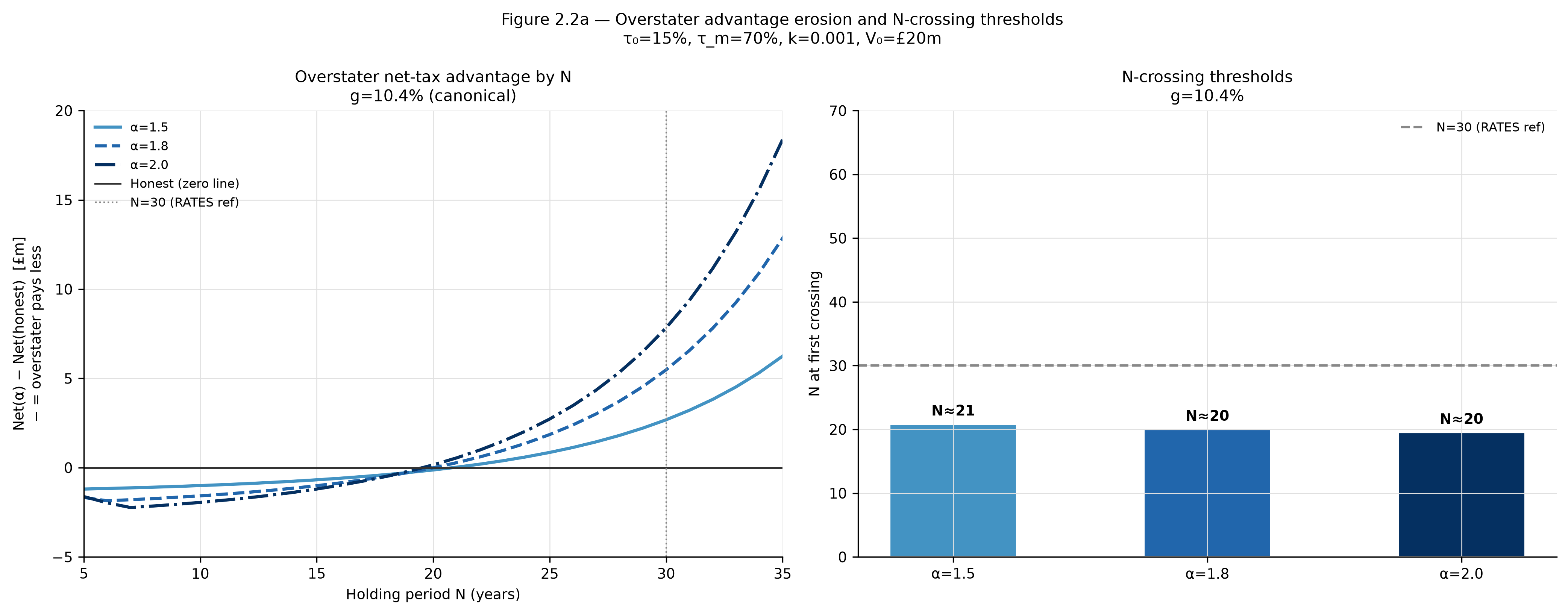
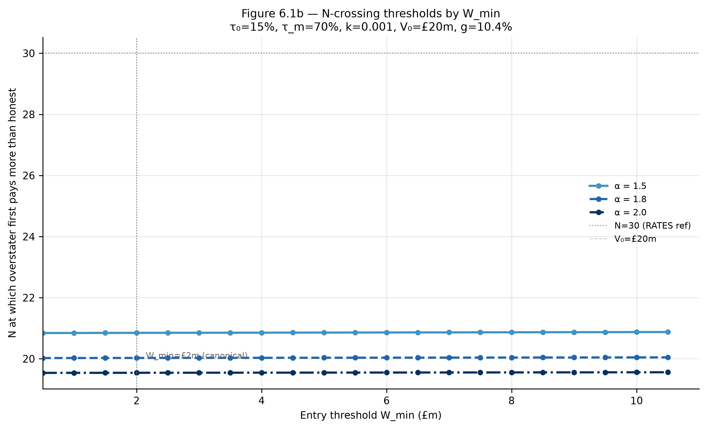
N-crossing threshold: The holding period N at which aggressive overstatement first becomes more expensive than honest declaration, marking the point at which the self-limiting correction has activated. In this paper, the threshold is tracked for \(\alpha\) = 1.5, \(\alpha\) = 1.8, and \(\alpha\) = 2.0; at canonical parameters these cross at approximately N = 21, 20, and 20 respectively (Table B.4.5).
SWEEPS.R: The parameter sweep dataset examining how the four rate-function parameters (\(\tau_0\), \(\tau_m\), k, \(W_{min}\)) affect fiscal outcomes (TCM coverage ratio and LRR fill year).
TCM coverage ratio: Average annual TCM net revenue over the capitalisation window as a share of average annual government expenditure; the primary measure of the mechanism’s fiscal scale.
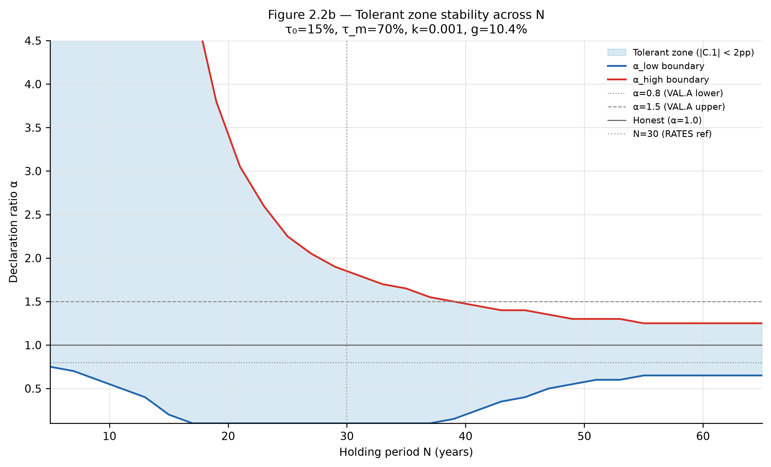
Tolerant zone: The \(\alpha\) band within which all declaration strategies produce approximately the same lifetime tax outcome as honest declaration (|C.1| < 2pp at canonical growth); a design feature absorbing valuation imprecision.
\(\tau_0\): The floor of the logistic rate function; the rate at which every taxpayer enters the system regardless of their position in the wealth distribution.
\(\tau_m\): The asymptotic ceiling of the logistic rate function; the rate the mechanism approaches but never reaches at extreme wealth.
Parameter separability: The property whereby the four rate-function parameters are doing largely independent jobs across the declaration-incentive and fiscal dimensions, such that calibrating one does not require simultaneous revision of the others.
Population-coverage parameter: A parameter whose primary consequence is determining how many taxpayers are subject to the mechanism, rather than what the mechanism does to those already in scope. \(W_{min}\) is the population-coverage parameter in the WDT rate function.
Understater penalty plateau ceiling: The maximum C.1 value reached by egregious understatement at high growth rates before the rate function saturates; the primary measure of deterrence at the extreme tail of the understatement distribution.
SWEEPS.V: The parameter sweep dataset examining how the four rate-function parameters affect declaration incentive properties (tolerant zone width, N-crossing threshold, understater penalty plateau ceiling).
\(W_{min}\): The wealth level below which the logistic rate function does not apply; determines the scope of the mechanism (who is subject to it).
1. Introduction
The architecture is fixed; the parameters are the Council’s to move. The architecture (delta base, symmetric refund, SWF, four valuation routes, three chambers) is protected by the enumerated structural clauses (GOV §5.2) and cannot be altered without triggering Tier 2 review and a permanent rebalancing cost.
This paper characterises the space within which that movement happens, drawing on two complementary sweep datasets. SWEEPS.V examines how the four rate-function parameters affect declaration incentive properties: tolerant zone width, self-limiting correction timing, understater deterrence strength. SWEEPS.R examines how the same parameters affect fiscal outcomes: coverage ratios and transition speed. Neither recommends values. Together they show the Council what it controls when it adjusts a given lever.
Two framing claims govern the paper. First, parameter setting is a policy question, not an optimisation problem: different settings reflect different judgments about speed, deterrence tail hardness, and taxable population scope. SWEEPS maps consequences; choices belong to the Council. Second, the WDT’s lever set is deliberately small. A small set of well-characterised parameters with observable consequences is preferable, on accountability and democratic legibility grounds, to a larger entangled set whose workings are opaque. The argument is in (SWEEPS §9).
This paper does not set parameters or recommend specific values. It is not a revenue paper; the quantitative extension of the fiscal sensitivity analysis is the natural RATES.A follow-on. The \(\tau_0\) tension identified in (SWEEPS §7) is characterised, not resolved.
Relationship to existing papers. SWEEPS draws on VAL, VAL.A, VAL.B, and RATES without revising them. It is the first paper to treat the Council’s calibration authority as its primary subject.
Confirmed figures. All SWEEPS.V and SWEEPS.R figures in (SWEEPS §3) to (SWEEPS §6) were generated at the confirmed canonical parameters (\(\tau_0\) = 15%, \(\tau_m\) = 70%, \(k\) = 0.001, \(W_{min}\) = £2m, N = 30) and are reported in SWEEPS.A. Quantitative values cited in the body are drawn from those confirmed tables. N = 30 is the demographic reference horizon: the approximate span from entry into scope at retirement (around age 60) to death (around age 90), representing a realistic upper bound on the time a taxpayer remains in the system. A taxpayer exits the system through death, emigration, or falling below the wealth threshold — N tracks years in the system, not the holding period of any individual asset.
2. What the Sweeps Are Measuring
This section establishes the five properties tracked across the two datasets. They are presented in interleaved order, moving from the mechanism’s treatment of the compliant middle through its handling of the overstater tail to its deterrence of the understater tail, with the fiscal dimension of each introduced alongside the declaration-incentive dimension.
2.1 The Tolerant Zone and Fiscal Coverage
The state’s interest in valuation accuracy is ultimately revenue. A declared value that differs modestly from true value does not meaningfully affect what the mechanism collects, because the basis update rule carries any gap forward and closes it over time. The tolerant zone formalises this: the \(\alpha\) band within which |C.1| < 2pp at canonical growth, where all declaration strategies produce approximately the same lifetime tax outcome as honest declaration. A wide tolerant zone is the correct design objective. The mechanism does not need valuation precision from the taxpayer population; it needs the tails to be expensive. Within the zone, imprecision is absorbed without consequence.
The fiscal counterpart is the TCM coverage ratio: average annual TCM net revenue over the capitalisation window as a share of average annual government expenditure. A parameter that widens the tolerant zone without materially reducing coverage is doing exactly what it should. A parameter that narrows the zone while also compressing coverage is making the mechanism more demanding without fiscal return.
2.2 The N-Crossing Threshold and LRR Fill Year
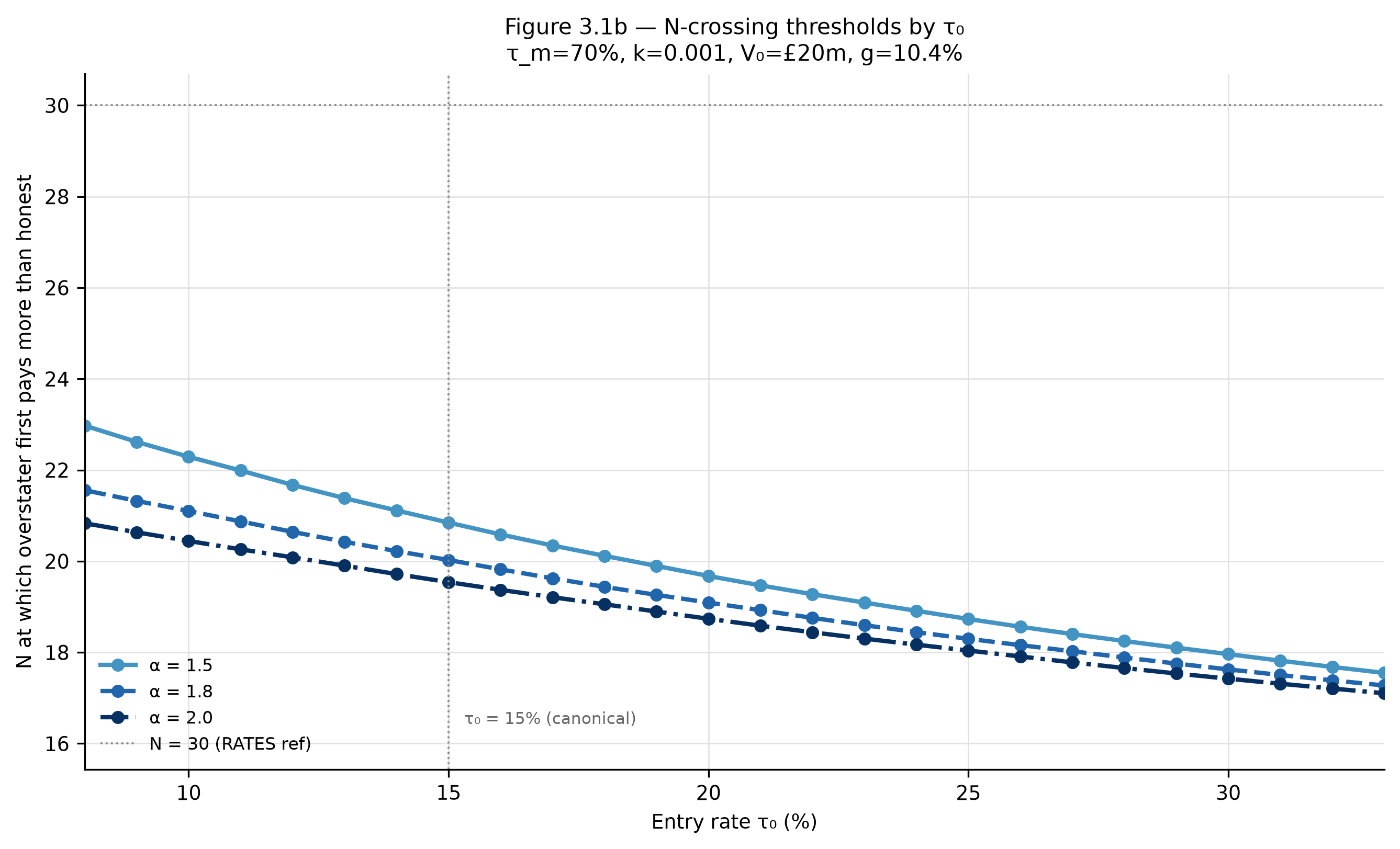
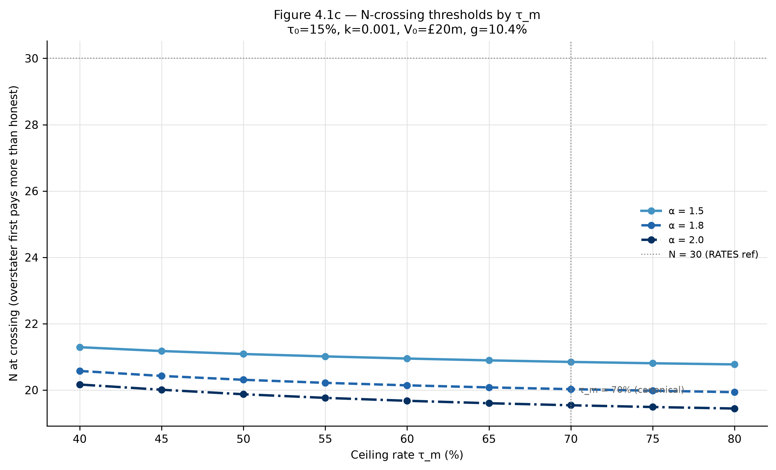
The N-crossing threshold is the number of years in the system at which a given degree of aggressive overstatement first becomes more expensive than honest declaration in nominal C.1 terms. N measures a taxpayer’s time in the system — it ends at death, emigration, or falling below the wealth threshold, not at the sale of any particular asset. This matters for how the threshold should be read: an overstater who has accumulated a C.1 advantage in the years before the crossing can only realise that advantage by exiting the system before N-crossing arrives. At canonical parameters all three tracked overstater levels cross well before the demographic horizon: \(\alpha\) = 1.5 at approximately N = 21, \(\alpha\) = 1.8 at N = 20, \(\alpha\) = 2.0 at N = 20 (Table B.4.5). A taxpayer who remains in the system past the crossing pays more in net tax than honest declaration would have cost — the advantage is gone, and the longer they remain, the larger the cost. By the canonical N = 30 horizon the correction has been active for roughly ten years.
A further qualification applies specifically to mild overstatement (\(\alpha\) = 1.5): while the nominal C.1 advantage is eliminated at the N-crossing, the NPV-adjusted C.12 metric established in (VAL.A §C.12) shows that the advantage does not survive discounting even before the crossing — periodic outflows are real early money while the sell-year refund is inflated late money. The N-crossing tracks the nominal incentive landscape; the economic conclusion (no genuine TW advantage from mild overstatement) holds at all N and all g, not only after the crossing point.
The N = 30 reference line used throughout the SWEEPS.V figures is the demographic reference horizon: the approximate span from entry into scope at retirement (around age 60) to death (around age 90), representing a realistic upper bound on time in the system. It is confirmed as the RATES capitalisation horizon in SWEEPS.A Table B.4.5, and appears on the charts as a temporal anchor, not a pass/fail threshold.
The fiscal counterpart is the LRR fill year: the first year the LRR balance reaches the three-year-expenditure floor, gating full Phase Two viability. Given that the N-crossing arrives well before the capitalisation horizon at canonical parameters, the relevant cross-dataset question for \(\tau_0\) is not whether the correction survives — it does, across the tested range — but how the pace of both the correction and the fiscal fill changes as \(\tau_0\) moves.
2.3 The Understater Penalty Plateau and What It Indicates
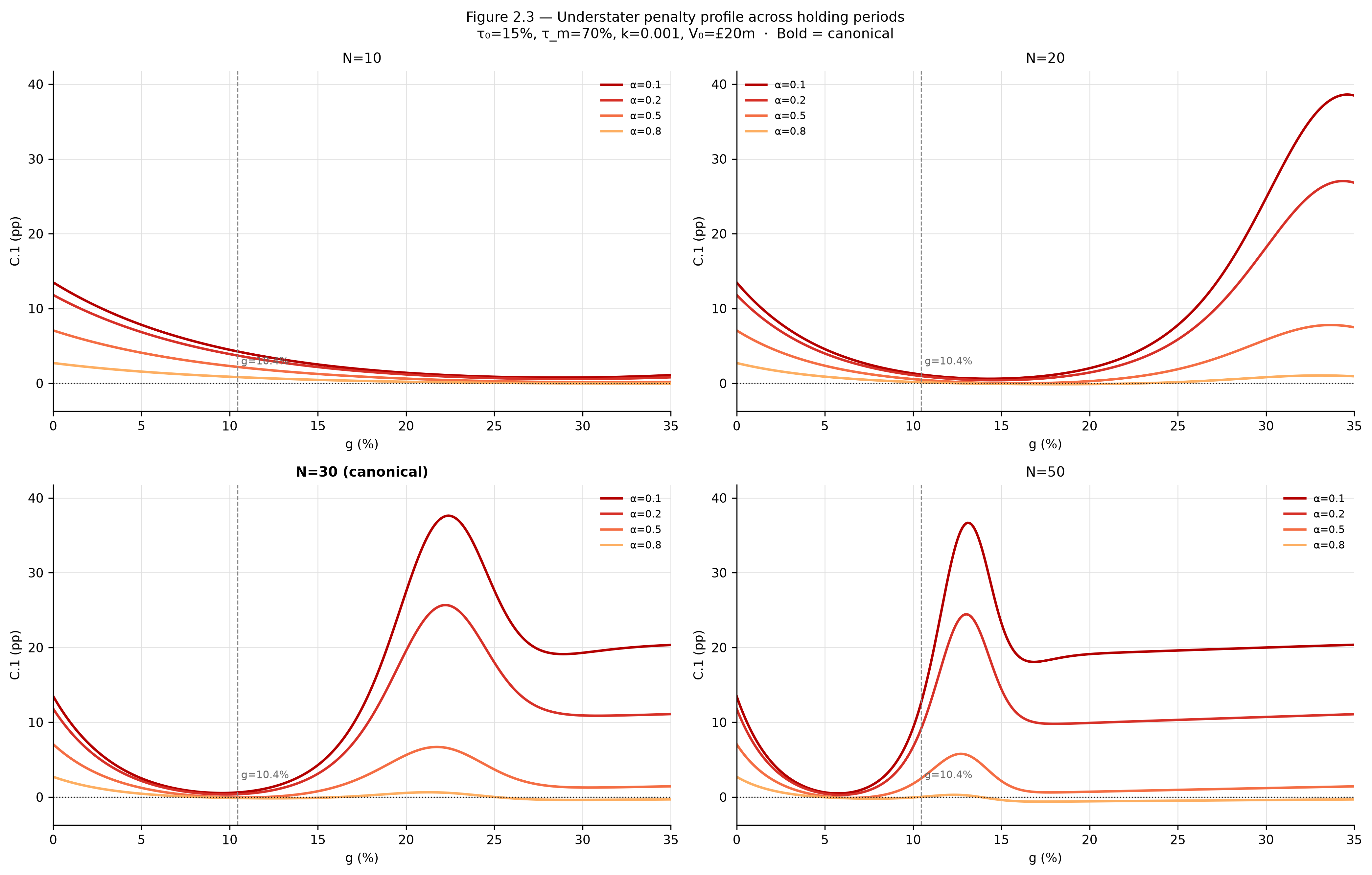
At canonical growth (\(g\) = 10.4%), the mechanism is approximately neutral to declaration strategy at some holding periods, but this is not N-invariant. At N = 30, C.1 is close to zero for moderate understatement; at shorter horizons some positive penalties remain; at N = 50, severe understatement produces substantially larger penalties even at canonical growth. Moderate understatement can also produce a very small negative C.1 in parts of the parameter space. At sufficiently long holding periods and high growth rates, mild understatement (\(\alpha\) = 0.8) produces a small, bounded tax advantage of approximately 1–2pp in the region shown.
The understater penalty plateau is the bounded high-growth level toward which C.1 settles after the curves pass through their intermediate-growth peaks. Under canonical parameters, severe understatement produces a pronounced transient peak at approximately \(g\) \(\approx\) 22%–23%, after which C.1 declines toward a substantially lower level. The plateau is therefore not the maximum C.1 the mechanism attains; the transient peak can be considerably higher. The ceiling is imposed by the logistic rate function at \(\tau_m\): once effective marginal rates approach that ceiling, further growth increases have progressively less effect on the relative penalty. Absolute tax liability continues to increase with terminal wealth, while the penalty relative to terminal wealth approaches a bounded level.
The N = 30 and N = 50 panels show very similar high-growth plateau levels and peak locations, suggesting the high-growth ceiling is relatively insensitive to additional holding period once the longer-horizon regime is reached. The canonical-growth region is nevertheless strongly N-dependent, and the growth rate at which the high-growth regime is reached also varies with holding period. The plateau value at a given \(\alpha\) is approximately N-invariant in the high-growth regime; the path into that regime is not.
Parameters governing the upper tail of the rate function, particularly \(\tau_m\), can alter the magnitude of the high-growth understater penalty while leaving the basic structure of the mechanism intact. The extent to which such parameters leave the lower-growth region quantitatively unchanged is an empirical property of the model rather than an assumption.
2.4 Reading the Two Datasets in Parallel
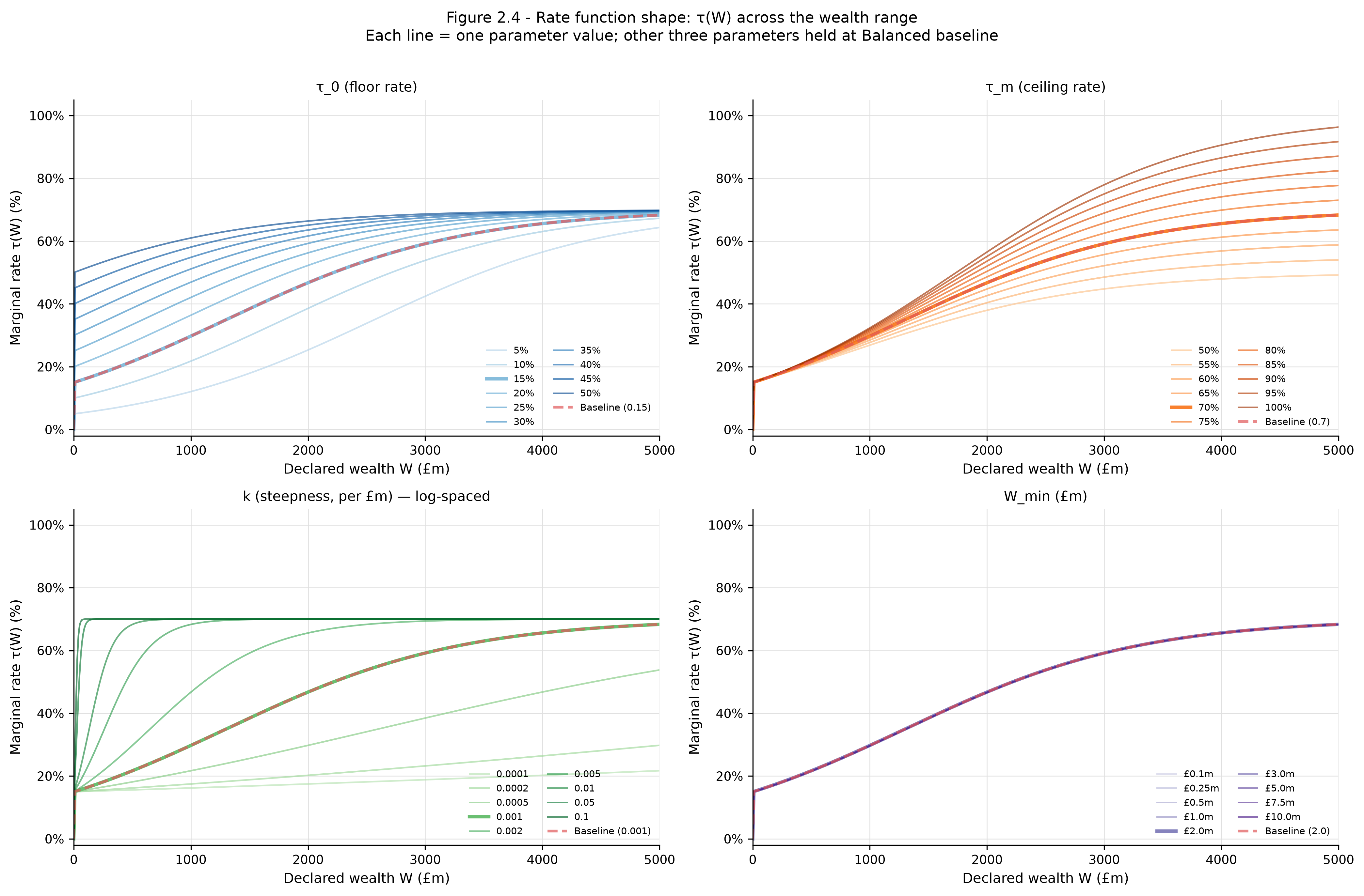
SWEEPS.V uses an individual-level cohort model; SWEEPS.R uses a population-level SSM and TCM. Their units are not directly comparable and they are not combined into a single metric here. The paper reads them in parallel throughout. Where both datasets agree on a parameter’s effect, the finding is robust across frameworks. Where one is silent on a dimension the other covers, that is stated explicitly. The \(\tau_0\) question — identified in (SWEEPS §7) as the most consequential calibration decision the Council faces — is one where the two datasets agree on direction but the parameter is doing several things at once, which is what makes it consequential.
3. \(\tau_0\) — The Entry Rate
\(\tau_0\) sets the floor of the logistic rate function at \(W_{min}\): the rate every taxpayer faces on their first pound of delta above the exemption threshold.
3.1 What \(\tau_0\) Controls on the Declaration Mechanism (SWEEPS.V)
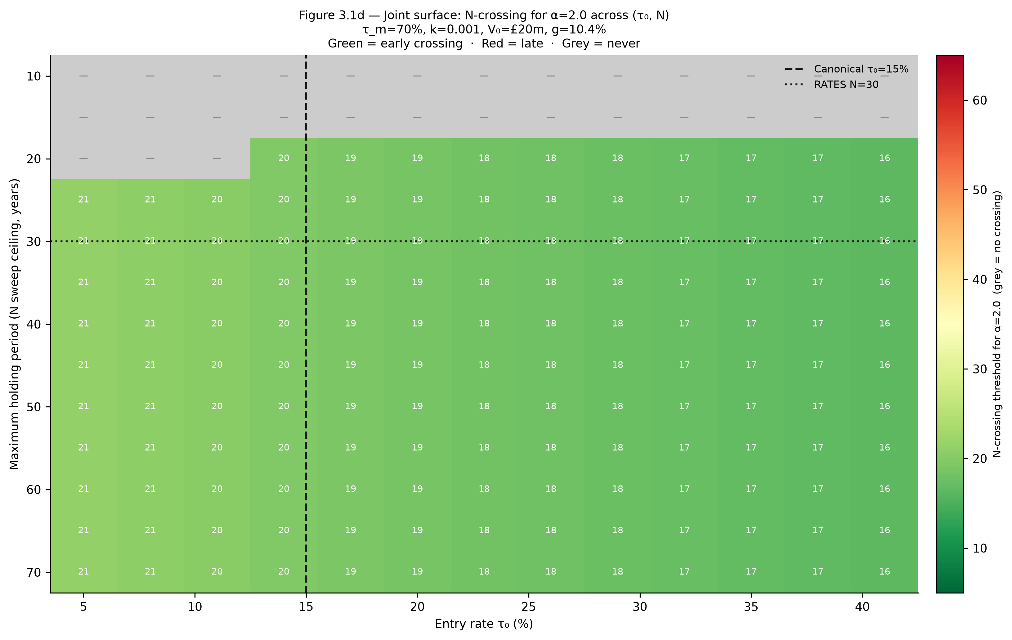
\(\tau_0\) is the primary lever for the N-crossing threshold. The joint surface (Table B.6) shows that raising \(\tau_0\) brings the correction earlier: at \(\tau_0\) = 5–8%, the \(\alpha\) = 2.0 crossing arrives at N = 21 (when the N sweep ceiling is sufficient to detect it); by \(\tau_0\) = 14–17% it has moved forward to N = 19–20; by \(\tau_0\) = 35–40% it reaches N = 16. A grey no-crossing region exists in the upper-left corner of the joint surface at low \(\tau_0\) and low N sweep ceilings — crossings are only detectable once the ceiling exceeds approximately N = 18–20 at the lowest floor rates. The direction is the reverse of rate-range compression intuition: higher \(\tau_0\) raises effective rates across the distribution, compressing the absolute advantage from overstatement and pushing the crossing earlier.
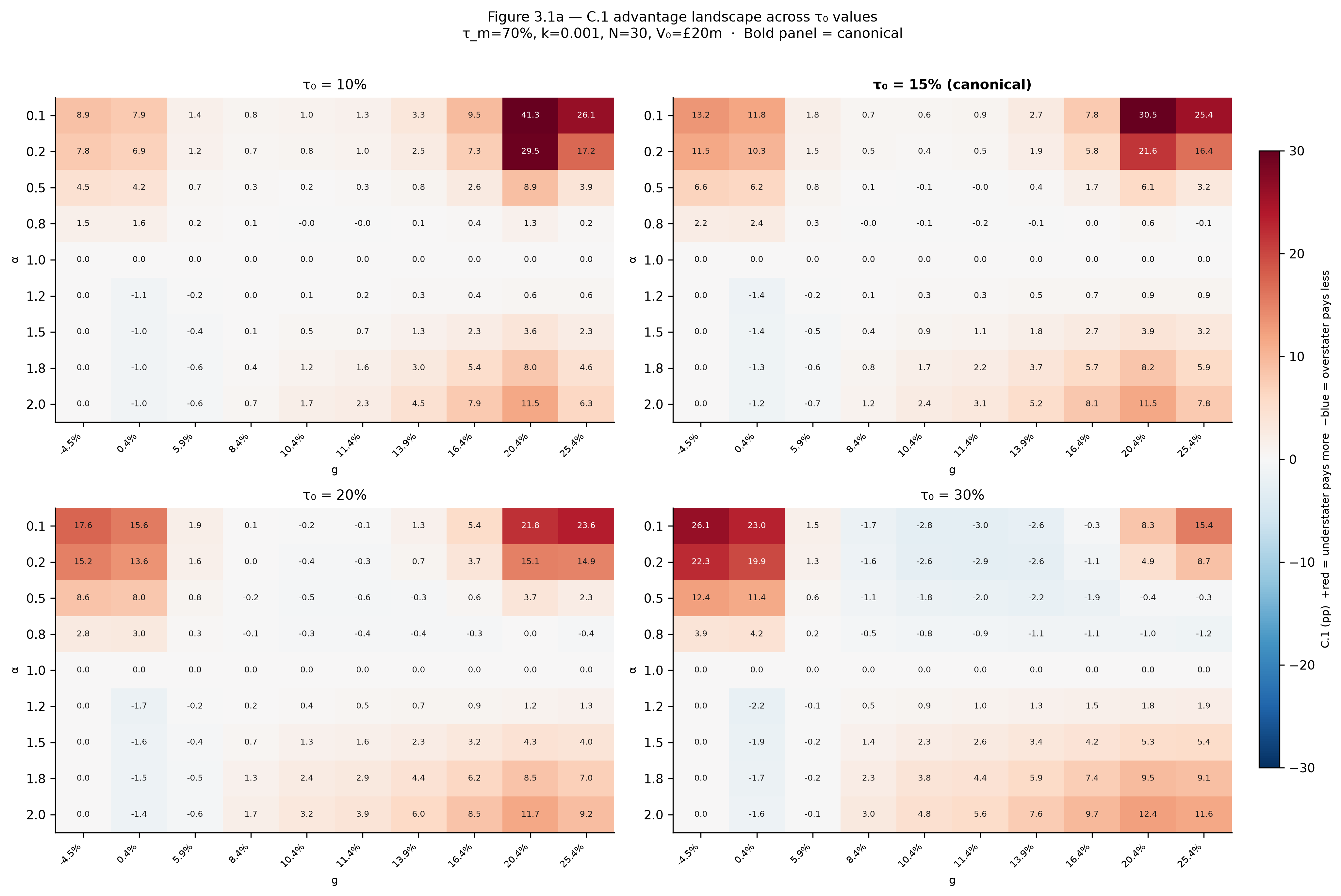
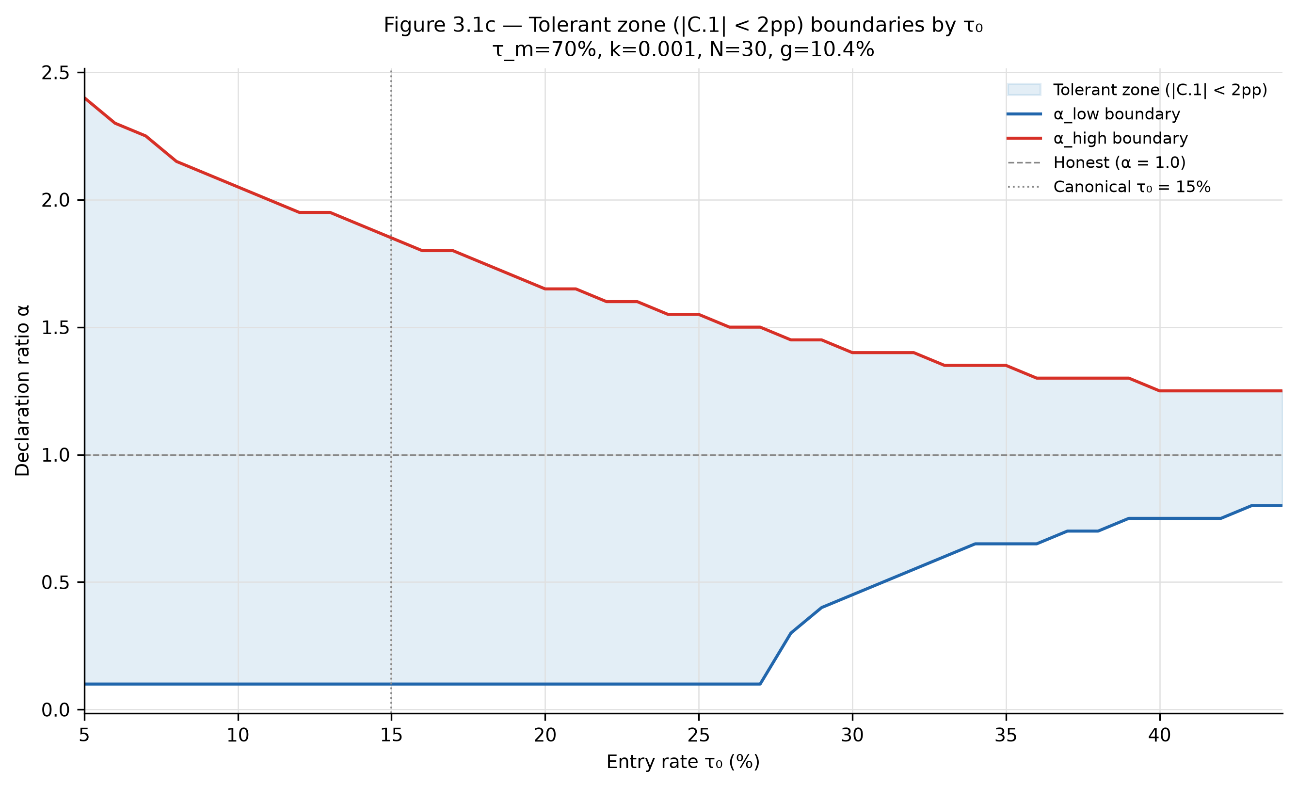
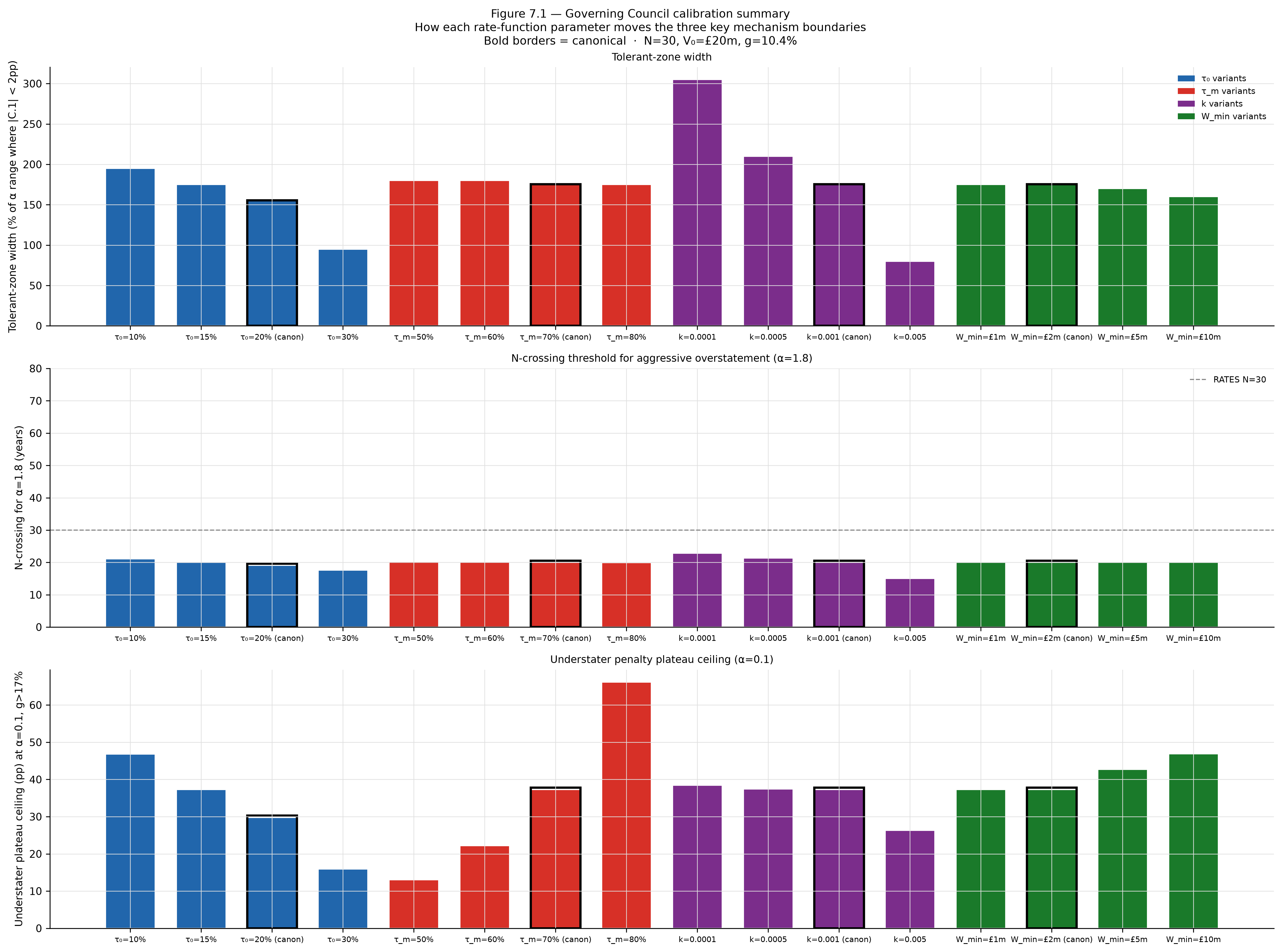
The tolerant zone width narrows progressively as \(\tau_0\) rises across the full tested range — from approximately 195% of the \(\alpha\) axis at \(\tau_0\) = 10% through approximately 155% at canonical \(\tau_0\) = 15% to approximately 95% at \(\tau_0\) = 30%. The upper boundary declines continuously rather than collapsing at a single threshold. This is a structural ceiling on how far \(\tau_0\) can be raised without materially narrowing the declaration equilibrium zone. At canonical \(\tau_0\) = 15% the upper boundary sits at approximately \(\alpha\) = 1.85, while the population-level declaration equilibrium sits near \(\alpha\) \(\approx\) 1.1 — the equilibrium is well inside the tolerant zone with substantial margin to spare. The narrowing with \(\tau_0\) is real, but the relevant comparison is not the zone’s absolute width but the gap between its boundary and the equilibrium the mechanism actually produces.
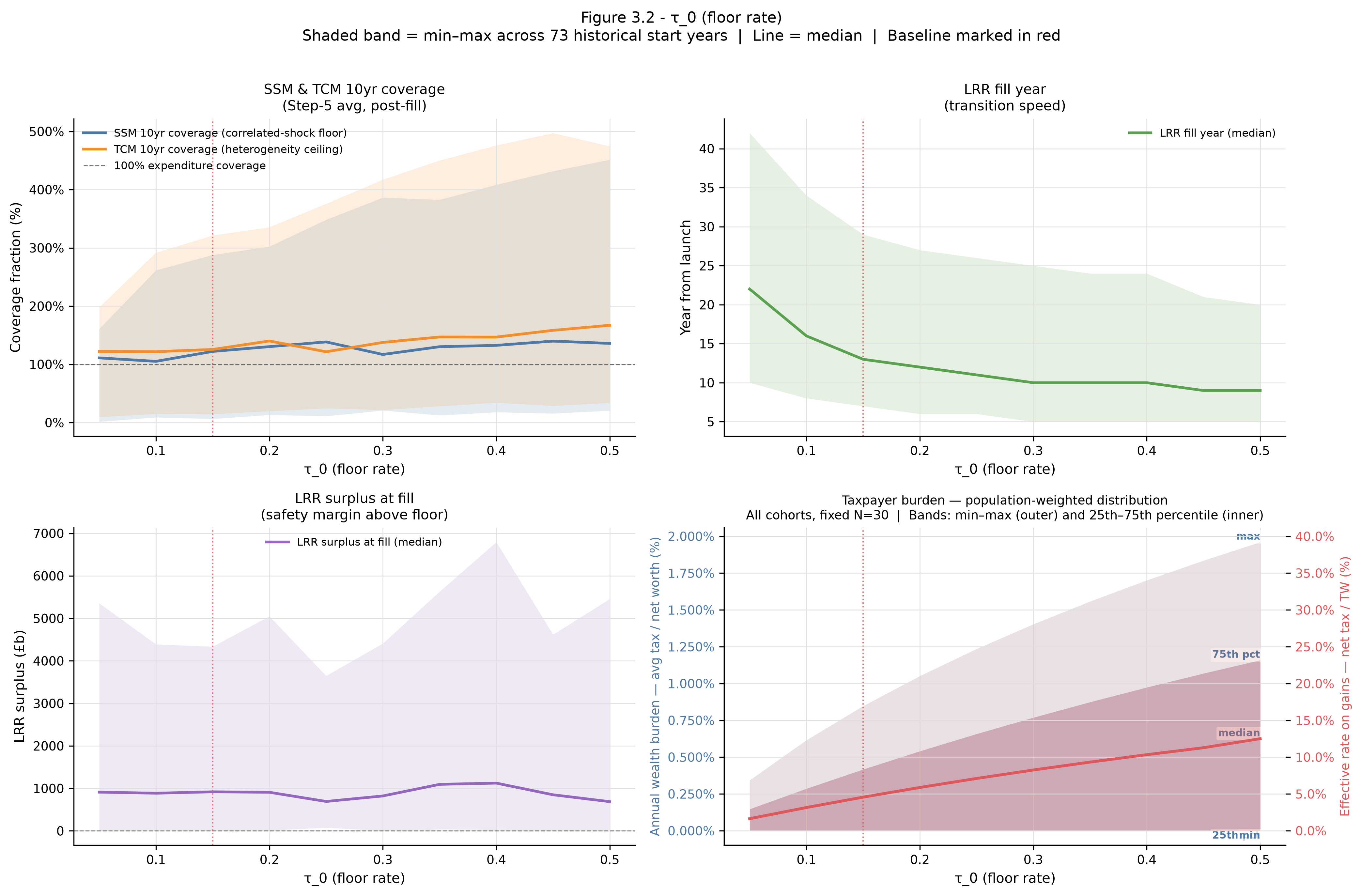
\(\tau_0\) has substantial secondary leverage on the understater plateau ceiling: the ceiling for \(\alpha\) = 0.1 falls from approximately 47pp at \(\tau_0\) = 10% to approximately 15pp at \(\tau_0\) = 30%, driven by the interaction between the floor rate and the rate ceiling. This is a larger secondary effect than previously characterised, though \(\tau_m\) remains the dominant lever for tail deterrence.
3.2 What \(\tau_0\) Controls on Fiscal Outcomes (SWEEPS.R)
\(\tau_0\) dominates the fiscal outcome hierarchy. At canonical \(k\) = 0.001, the effective rate across all ten wealth brackets sits near the logistic floor throughout the capitalisation window: the logistic midpoint at canonical parameters is approximately £1,387m, well above the top bracket’s mean entry wealth of £139.6m. Because the brackets never meaningfully ascend the logistic curve during the capitalisation period, \(\tau_0\) directly determines what every bracket pays. It is not acting as a floor that other parameters build on; it is, for the modelled population, approximately the whole rate.
A 10pp increase in \(\tau_0\) reduces the median LRR fill year substantially at the lower end of the tested range — from 22 years at \(\tau_0\) = 5% to 13 years at \(\tau_0\) = 15%, a 9-year reduction — with sensitivity flattening to approximately 2 years per 10pp through the middle of the sweep. Median coverage is already above 100% expenditure coverage at canonical parameters and rises further with \(\tau_0\), from approximately 110% at \(\tau_0\) = 5% toward 160% at \(\tau_0\) = 50% — the SSM and TCM medians track closely together across the full sweep.
The 2006 worst-case scenario shows an anomaly at the \(\tau_0\) = 20–25% transition: LRR fill year falls from 26 to 25 years while the LRR surplus at fill drops from £1,999b at \(\tau_0\) = 20% to £973b at \(\tau_0\) = 25%. This reflects the capitalisation window at \(\tau_0\) = 20% closing into a lower-return portion of the 2006 return sequence, compressing the surplus without substantially advancing fill timing. The rate effect then dominates cleanly above \(\tau_0\) = 25%.
3.3 What the Council Is Calibrating When It Sets \(\tau_0\)
\(\tau_0\) is architecturally unusual: it is the one parameter where fiscal outcomes and declaration incentives move in the same direction. Most tax parameters involve a tension between revenue performance and behavioural consequences — raising a rate tends to improve one while complicating the other. \(\tau_0\) does not. Raising the floor accelerates LRR capitalisation, brings the overstater correction earlier, and raises effective rates on understaters throughout the distribution. There is no \(\tau_0\) value at which the mechanism becomes less self-correcting, and no \(\tau_0\) value at which fiscal capitalisation slows while the correction speeds up. The two datasets agree on direction throughout the tested range. That alignment is the parameter’s defining property and the reason it is the most consequential calibration decision the Council faces.
What it does force is a choice about entry burden. The cooperative-entry rationale for the mechanism favours a low initial claim on wealth increments: a floor rate that reads as proportionate rather than extractive is more likely to secure the political and behavioural cooperation on which Phase One depends. Higher \(\tau_0\) is better on speed by every measurable dimension in the sweep data; whether it is better on sustainability depends on how the taxable population and its political representatives respond to the entry rate they first encounter. The sweep data cannot answer that question. Phase One is the test.
The policy question the Council faces is therefore not which dimension to sacrifice — both move together — but how fast to go, and at what initial burden level Phase One is most likely to establish the cooperative norm the mechanism depends on.
4. \(\tau_m\) — The Ceiling Rate
\(\tau_m\) is the asymptotic ceiling of the logistic rate function. Where \(\tau_0\) sets the floor every taxpayer encounters on entry, \(\tau_m\) sets the upper bound that only the wealthiest positions approach over long holding periods.
4.1 What \(\tau_m\) Controls on the Declaration Mechanism (SWEEPS.V)
\(\tau_m\) is the primary lever for understater penalty deterrence at the extreme tail. Its effect on tolerant zone width is near-zero — the zone’s boundaries are largely insensitive to the ceiling rate across the full tested range. Its leverage on the N-crossing threshold is minimal: a 40pp sweep of \(\tau_m\) (from 40% to 80%) moves the \(\alpha\) = 2.0 crossing by approximately 1 year, compared to approximately 3 years for an equivalent \(\tau_0\) sweep across a comparable range.
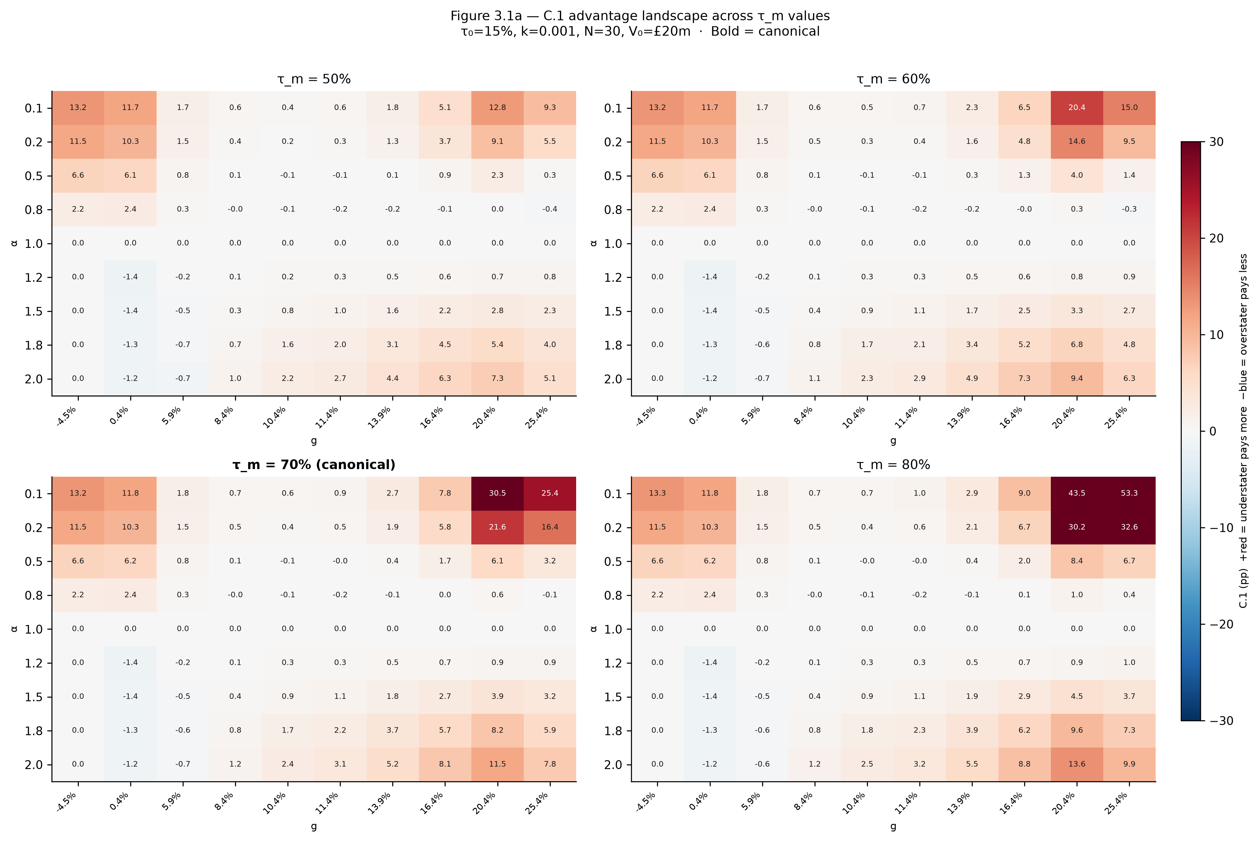
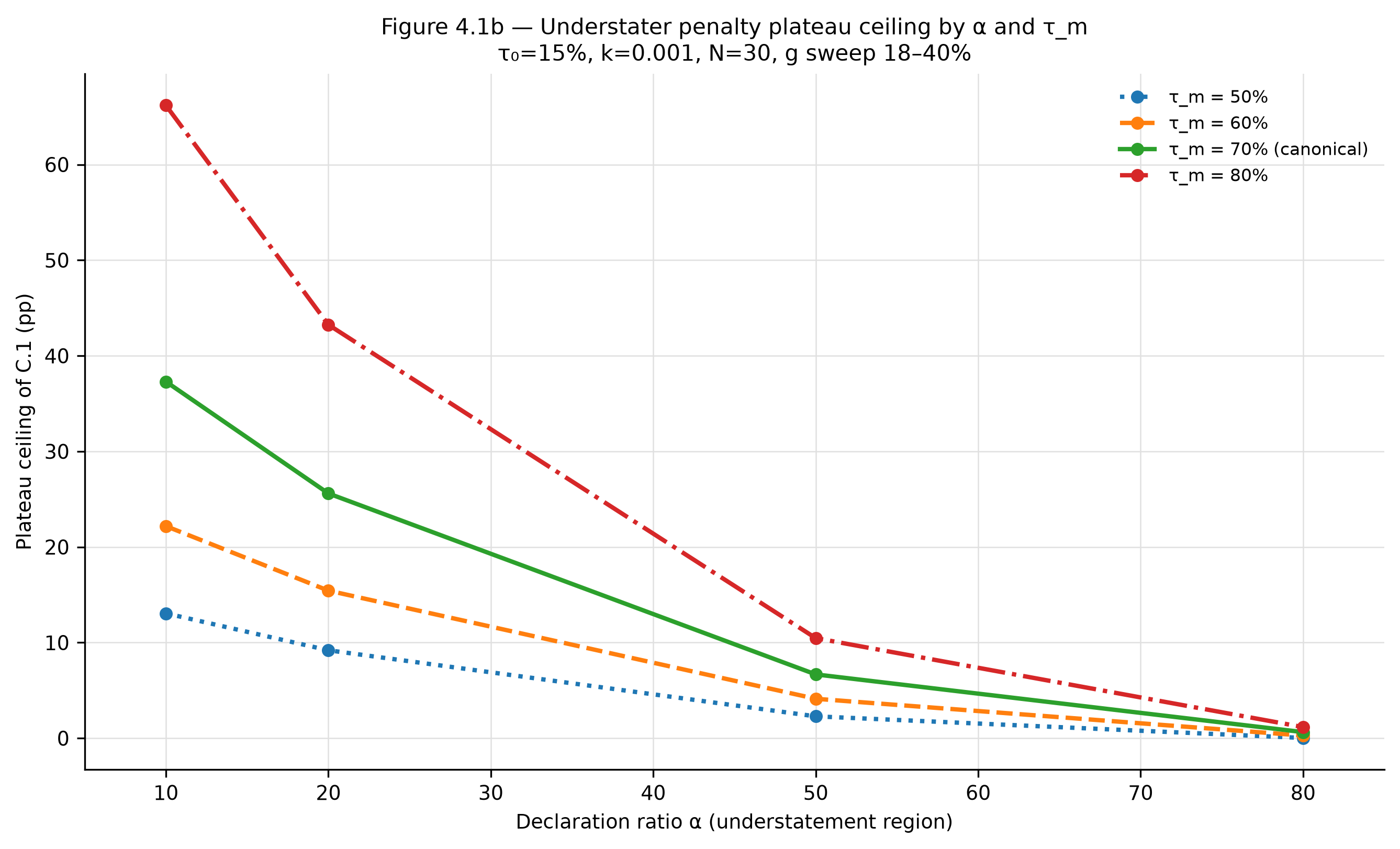
The strong effect is concentrated entirely on the plateau ceiling. At \(\tau_m\) = 50% the \(\alpha\) = 0.1 penalty reaches approximately 12pp at the high end of the growth sweep; at \(\tau_m\) = 80% it reaches approximately 65pp. The peak occurs near \(g\) \(\approx\) 22–23% at canonical N = 30 rather than at the highest tested growth rate, reflecting the interaction between the rate ceiling and the growing terminal-wealth denominator. At \(\alpha\) = 0.8 (mild understatement) all \(\tau_m\) variants cluster near zero regardless of ceiling rate. \(\tau_m\) has essentially no effect on the compliant middle or the moderate overstater; its consequence is specific to the far tail of the understatement distribution.
4.2 What \(\tau_m\) Controls on Fiscal Outcomes (SWEEPS.R)
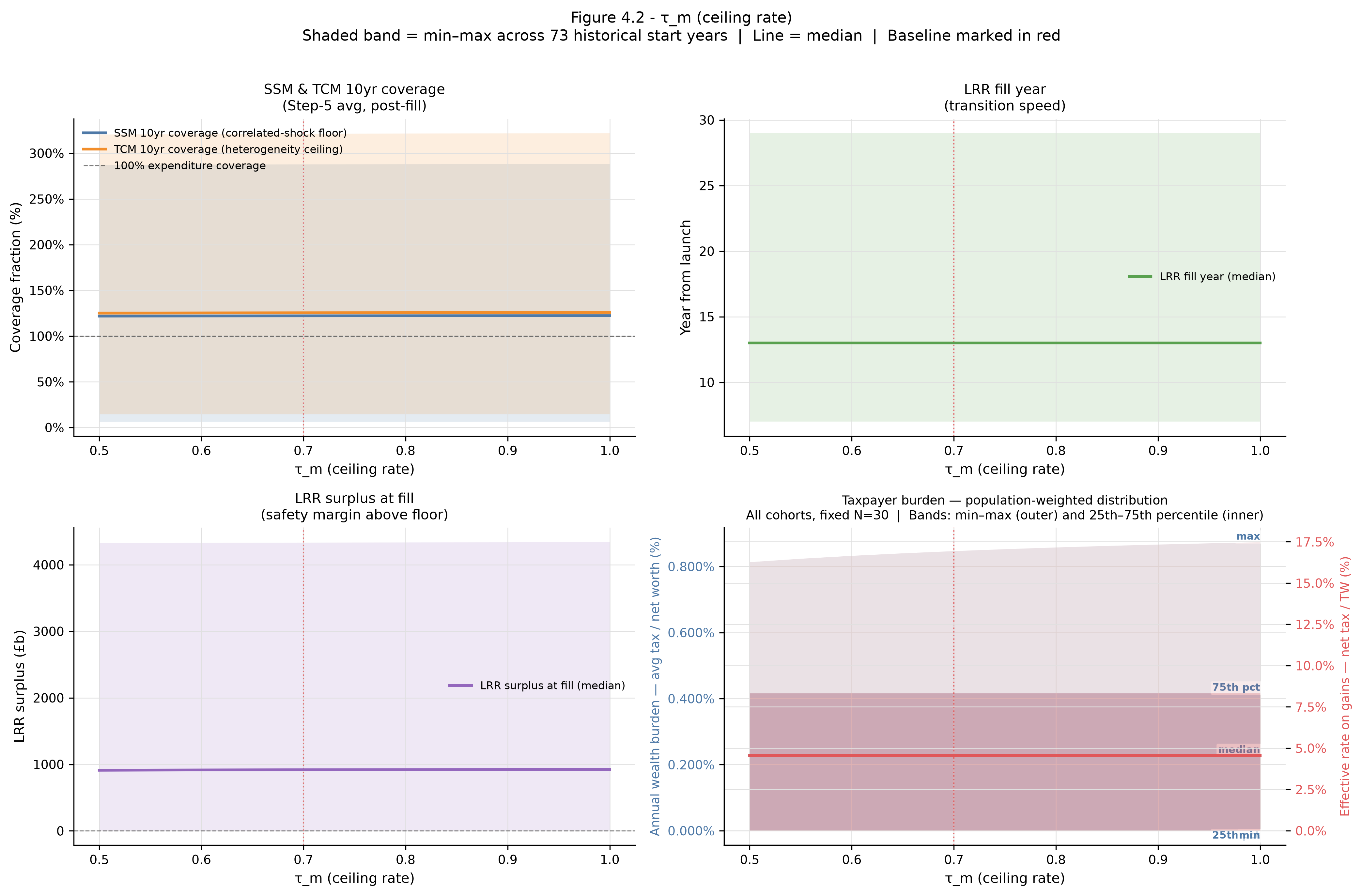
For the modelled population, \(\tau_m\) is fiscally inert. SWEEPS.R coverage and fill-year outputs are flat across the full \(\tau_m\) sweep from 50% to 100%. At canonical k, no wealth bracket approaches wealth levels where the ceiling constrains the effective rate during the capitalisation window: the top bracket enters at a mean wealth of £139.6m and reaches approximately £1,266m at year 30, at which point \(\tau(W)\) = 32.9% under \(\tau_m\) = 70% — well below the ceiling. That bracket accounts for approximately 0.2% of aggregate capitalisation-window revenue. Changing \(\tau_m\) from 50% to 100% shifts its contribution by roughly 15%, which is negligible in aggregate.
\(\tau_m\) becomes fiscally relevant when the taxable population includes sustained multi-decade ultra-high-net-worth holdings above £500m–£1bn. The current bracket structure does not reach that territory. Any future recalibration of \(k\) that places more of the population on the steep portion of the logistic curve would change this; the \(k\) sweep in SWEEPS.A confirms the finding holds at canonical \(k\) = 0.001.
4.3 What the Council Is Calibrating When It Sets \(\tau_m\)
\(\tau_m\) is the one rate parameter where the two datasets give unambiguous, non-conflicting guidance. On the declaration side it is the egregious-understater deterrence lever. On the fiscal side it is inert for the current population. A Council calibrating \(\tau_m\) is setting the severity of the mechanism’s response to the most dishonest declarations, at essentially zero revenue cost or benefit. The separability is complete: the parameter has one job on the declaration side and nothing on the fiscal side.
The corrected plateau ceiling figures bear on whether the canonical \(\tau_m\) = 70% is adequately calibrated on that one job. At canonical settings (\(\tau_m\) = 70%), the \(\alpha\) = 0.1 penalty peaks at approximately 37pp near \(g\) \(\approx\) 22–23%; raising \(\tau_m\) to 80% raises the peak to approximately 65pp. To make the magnitude concrete: for a taxpayer entering at £500m growing at 22%, a 37pp penalty represents an excess cost of approximately £185m relative to honest declaration at the peak — the mechanism is imposing very large absolute consequences on the most egregious understatement at high growth rates. The question the Council faces is whether that is the right ceiling, not whether the mechanism is operating. The corrected figures make the gap between 70% and 80% clearly visible, and the fiscal cost of moving to 80% is near-zero while the deterrence gain is substantial. That asymmetry is directly relevant to the calibration decision.
Chamber positions on \(\tau_m\) reflect competing preferences about tail deterrence rather than competing fiscal interests: TP tends toward lower, FS toward higher, DR toward higher when the labour dividend is the salient political object. The fiscal stakes of the disagreement are near-zero for Phase One. The chamber conflict about \(\tau_m\) is real; its material consequence for the mechanism’s fiscal performance is not.
5. \(k\) — The Steepness Parameter
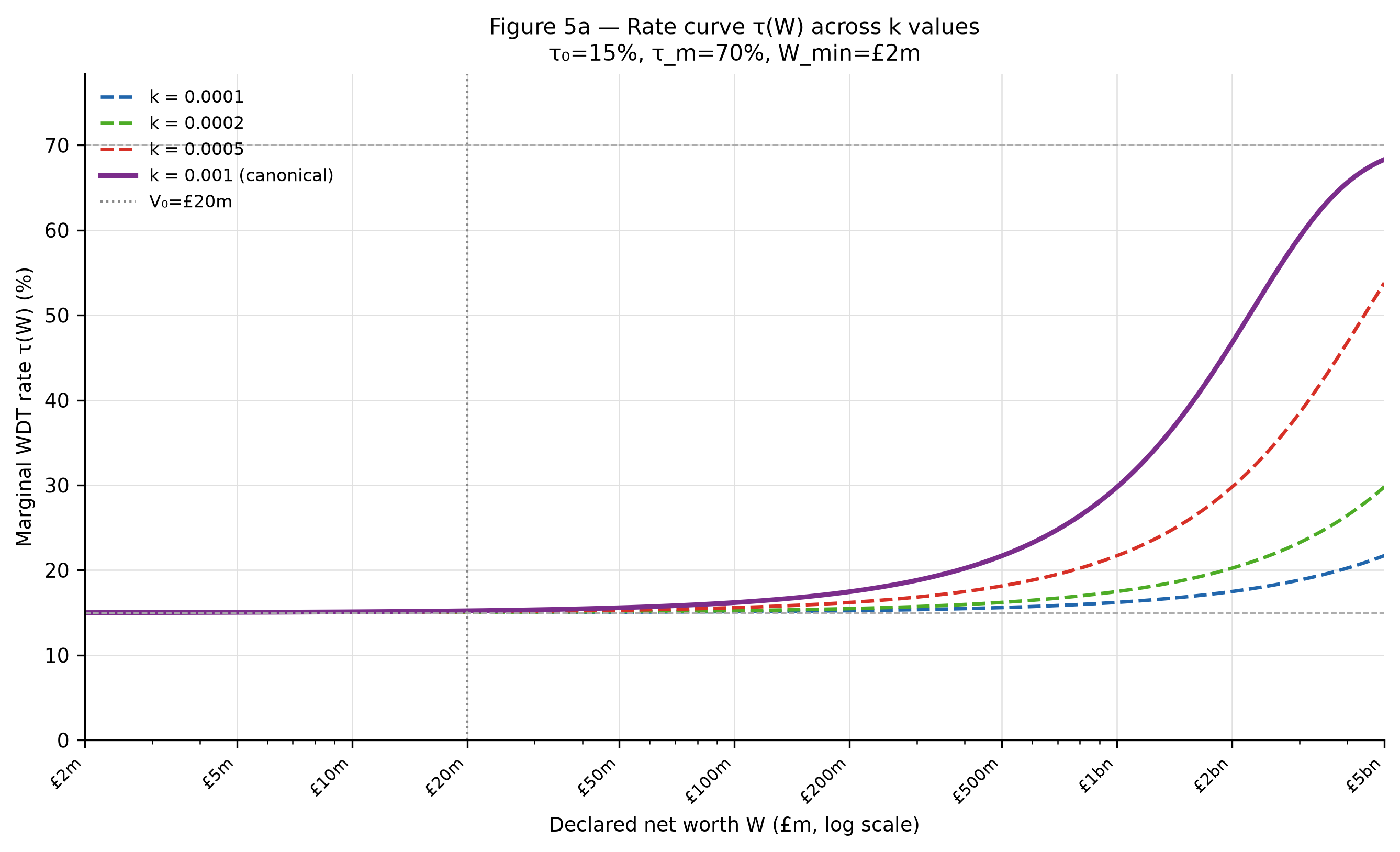
k controls the rate at which the logistic function rises from \(\tau_0\) toward \(\tau_m\) as wealth increases above \(W_{min}\). It determines where in the wealth distribution the mechanism becomes meaningfully progressive, and consequently how much of the rate curve’s available range any given taxpayer actually experiences.
5.1 What \(k\) Controls on the Declaration Mechanism (SWEEPS.V)
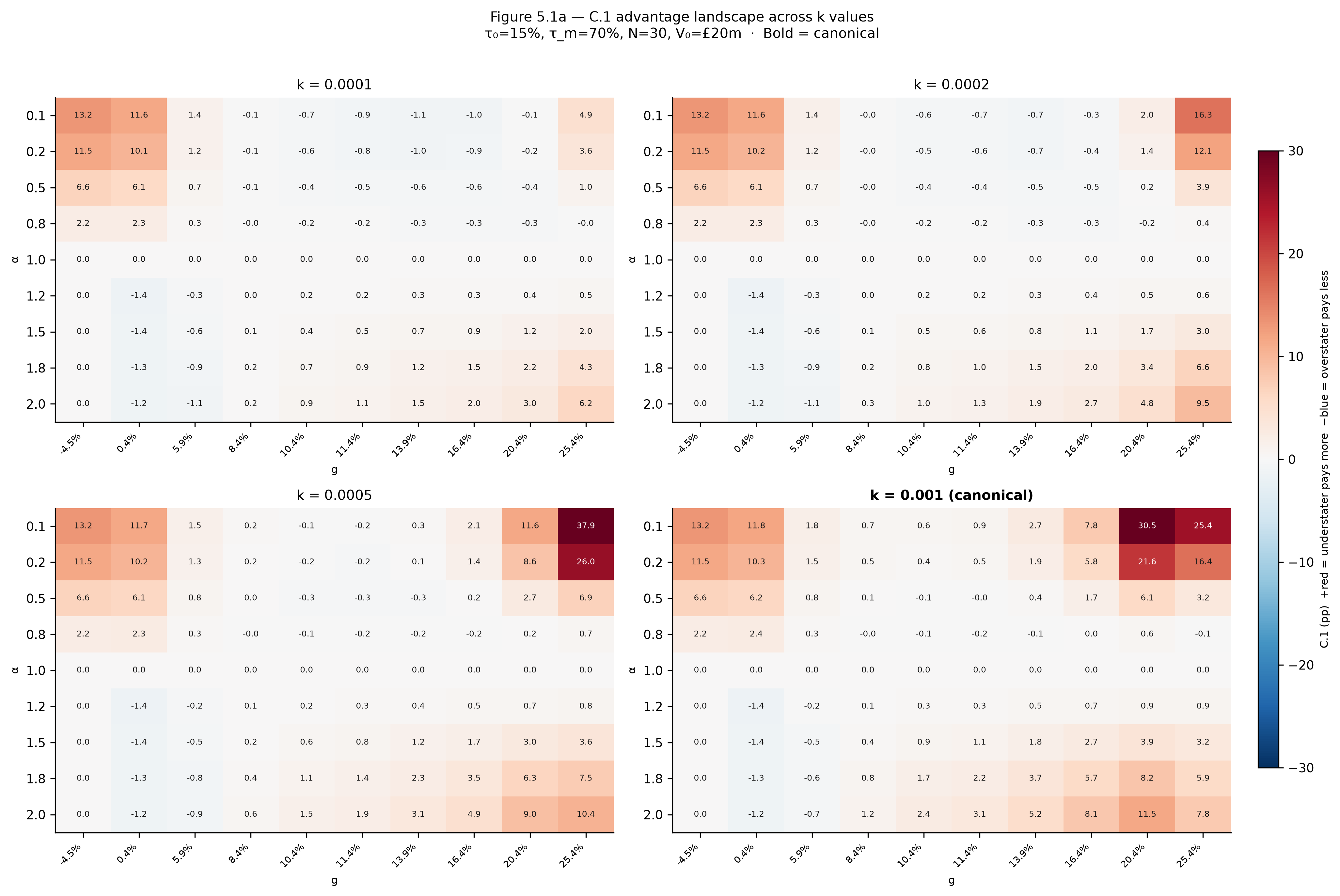
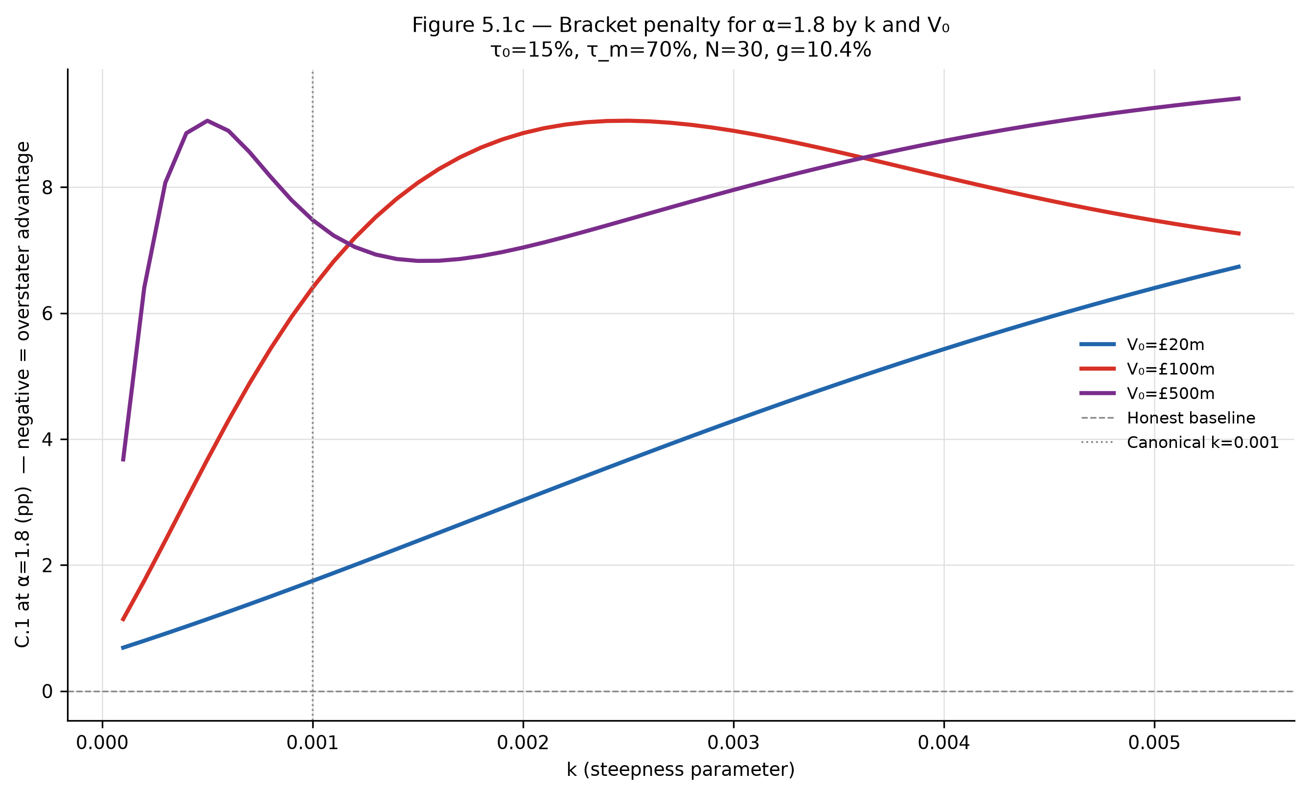
k is the primary lever for tolerant zone width. At \(k\) = 0.0001 the C.1 landscape is nearly flat: the \(\alpha\) = 0.1 understater penalty at the highest growth rate tested reaches approximately 4.9pp, and at high growth rates overstater cells show small negative C.1 values — a mild advantage that disappears as \(k\) rises. By \(k\) = 0.005 the zone has narrowed substantially: understater penalties intensify and the tails sharpen in both directions. The sign pattern across the heatmap is stable throughout: understater rows remain costly regardless of \(k\) value. Overstater rows show positive C.1 values at canonical growth throughout the sweep — the correction is active at N = 30 across all tested steepness values — and intensify with rising \(k\). At very low k, magnitudes are small because the rate curve barely rises across the wealth distribution. At high k, the tails intensify without penalising the compliant middle — \(k\) sharpens the mechanism at the extremes without narrowing the forgiving centre.
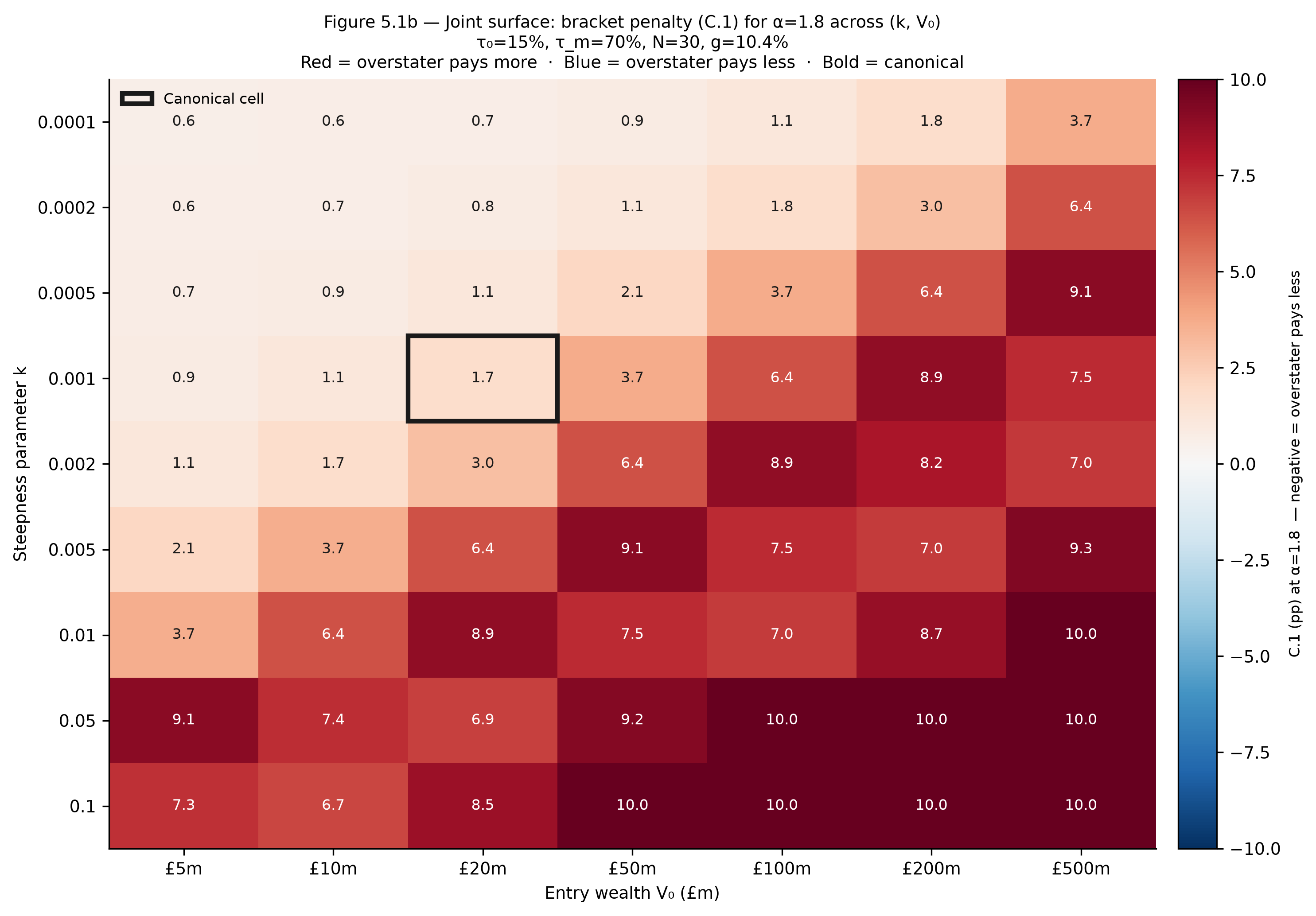
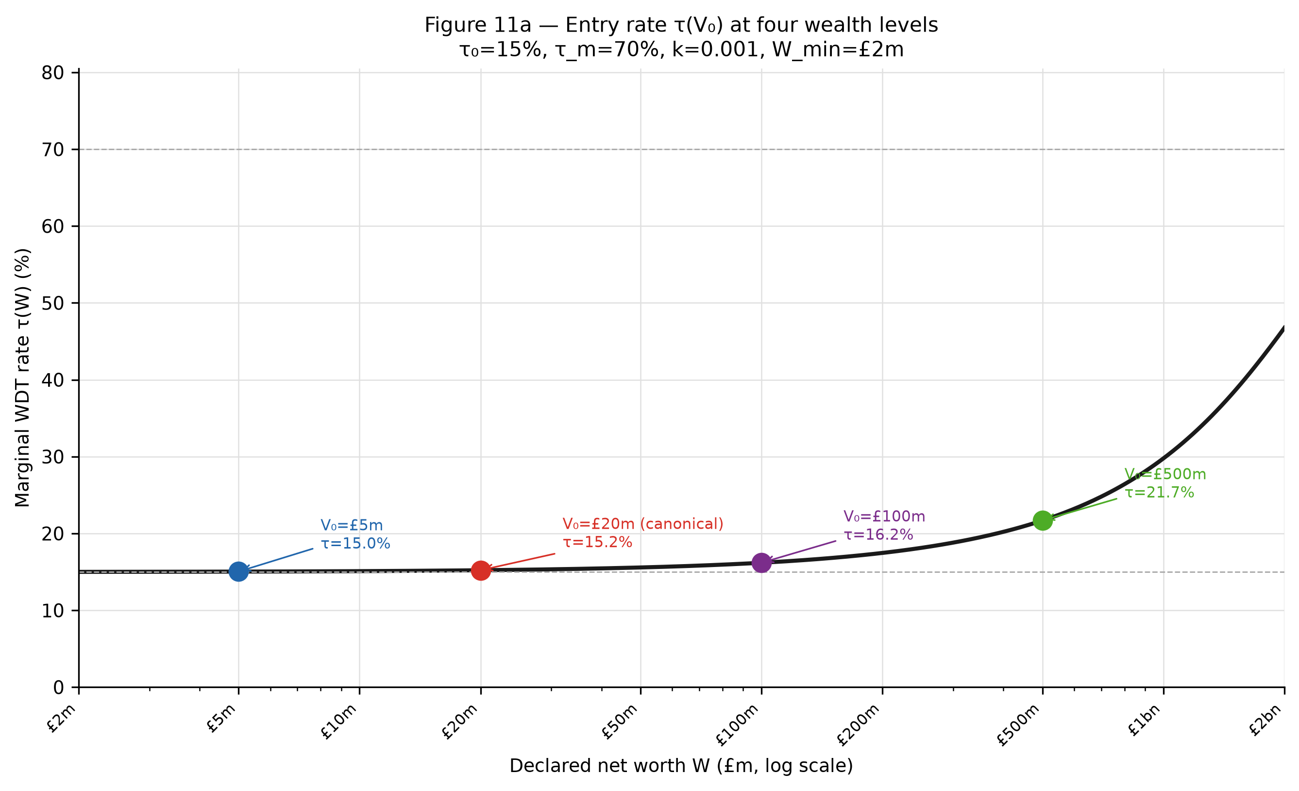
The \(k\) × \(V_0\) interaction is material. Near-threshold taxpayers at \(V_0\) = £20m sit on the flat lower portion of the rate curve regardless of k; their declaration incentives are largely insensitive to steepness. Taxpayers at \(V_0\) = £500m sit on the curve’s slope where \(k\) matters substantially — the same overstatement ratio produces a much larger bracket movement for a wealthier position. The joint surface (Fig S4.2) shows C.1 at \(\alpha\) = 1.8 positive (correction active) across the full \(k\) × \(V_0\) grid at canonical growth and N = 30: the self-limiting mechanism has activated for overstaters at all tested wealth and steepness combinations at this holding horizon, with the correction intensifying at higher \(k\) and higher \(V_0\).
5.2 What \(k\) Controls on Fiscal Outcomes (SWEEPS.R)
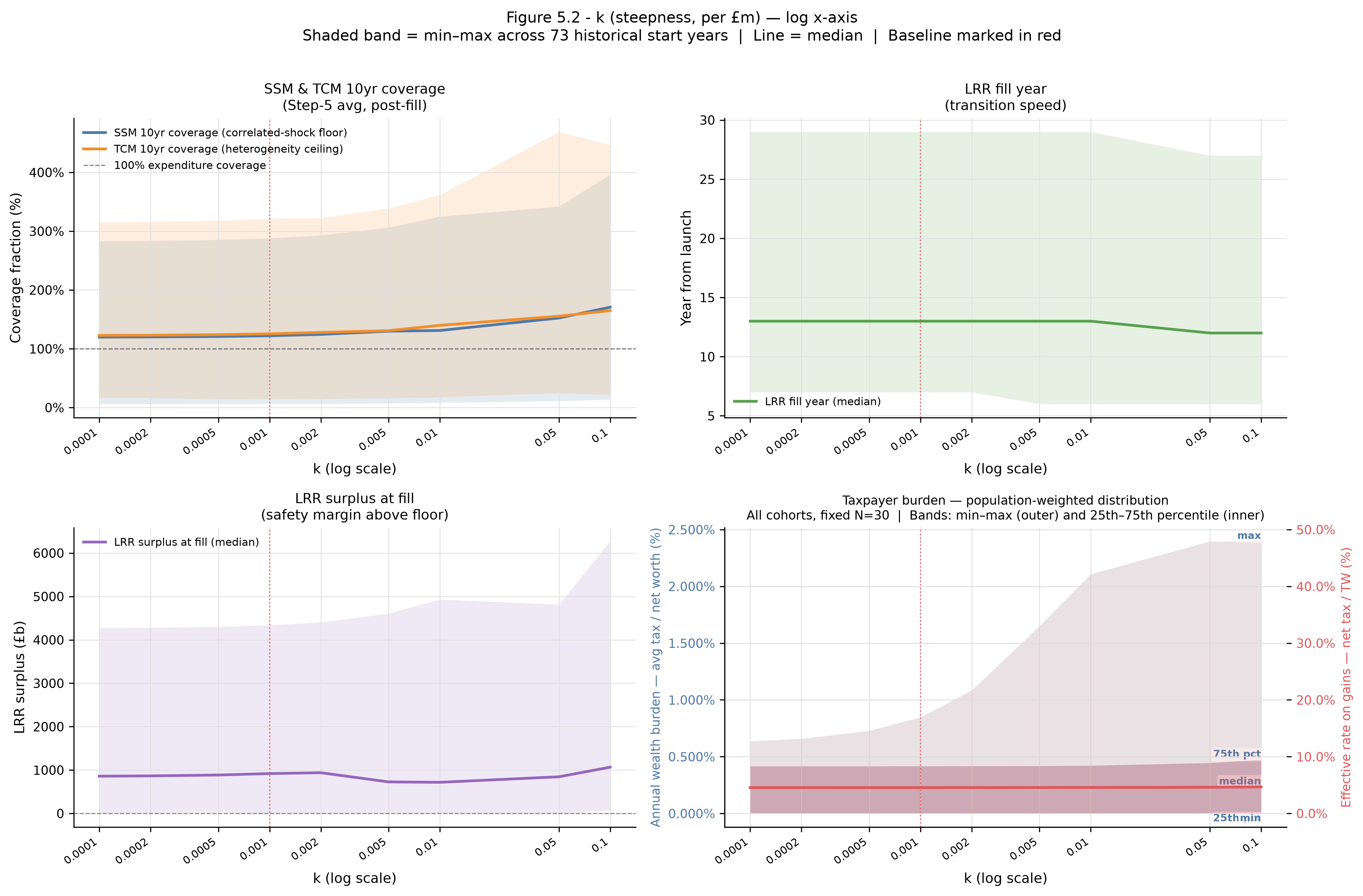
k matters at the upper end of realistic values. Below \(k\) \(\approx\) 0.005 the function rises so slowly that bracket-level tax burden is barely affected and TCM coverage barely moves. Above \(k\) = 0.01 the top brackets begin to approach the logistic midpoint within the capitalisation window, producing measurable TCM coverage improvements of approximately 4–5pp at \(k\) = 0.1 relative to baseline. The LRR fill year is largely unaffected until \(k\) reaches ranges where bracket midpoints are approached. Within the hierarchy established in (SWEEPS §3) to (SWEEPS §4), \(k\) is the third fiscal lever after \(\tau_0\) and \(W_{min}\), and conditionally so — its fiscal consequence is limited unless the bracket structure extends significantly further up the wealth distribution.
Success remains 100% across all nine tested \(k\) values (0.0001 to 0.1). The prior finding of reduced success rates at \(k\) = 0.05 (96%) and \(k\) = 0.1 (90%) was an artefact of the since-corrected budget_growth = 4.51%; at the corrected 4.51% the smaller LRR target grows more slowly, keeping LRR fill within reach across all historical start years even at high k. Raising \(k\) therefore does not threaten solvency guarantees within the tested range; the fiscal and mechanism-integrity dimensions of \(k\) remain separable. The canonical \(k\) = 0.001 sits in the flat lower portion where fiscal sensitivity is minimal.
5.3 What the Council Is Calibrating When It Sets k
k is the progressivity lever. At canonical \(k\) = 0.001 the logistic midpoint sits at approximately £1,301m, placing most of the modelled taxable population in the near-flat portion of the curve. Within that range the mechanism is approximately proportional: taxpayers face similar effective rates regardless of where in the distribution they sit. The mechanism becomes progressive only at extreme wealth, where the curve’s slope is encountered. A Council raising \(k\) is moving that transition point downward, making progressivity bite at lower wealth levels, with modest fiscal consequence unless the bracket structure extends to the newly affected range.
This is also \(k\)’s key design virtue: raising it sharpens the mechanism precisely where sharpening is warranted — at the extreme tails of the declaration distribution — while leaving the compliant middle largely undisturbed. At low \(k\), penalties are small everywhere and the mechanism is approximately toothless at the extremes. At higher \(k\), understater penalties and overstater corrections both intensify, but the interior of the heatmap — moderate \(\alpha\), the range where most taxpayers will sit — remains near-zero. \(k\) is the lever that makes the mechanism more demanding without making it less forgiving.
The intra-TP division that \(k\) produces differs structurally from the TP/FS opposition other parameters generate. Near-threshold TP members are largely indifferent to k: their bracket position is barely affected by steepness changes. Mid-tier TP members face the sharpest rate increase from a \(k\) rise and have the strongest reason to oppose it. Ultra-HNWI TP members are already near \(\tau_m\) regardless of \(k\) and are relatively indifferent in the other direction. This three-way internal split prevents TP from presenting a unified front on k, which is the correct outcome: within-TP heterogeneity about progressivity reflects actual differences in position on the rate curve rather than a collective interest the chamber can articulate coherently.
6. \(W_{min}\) — The Exemption Threshold
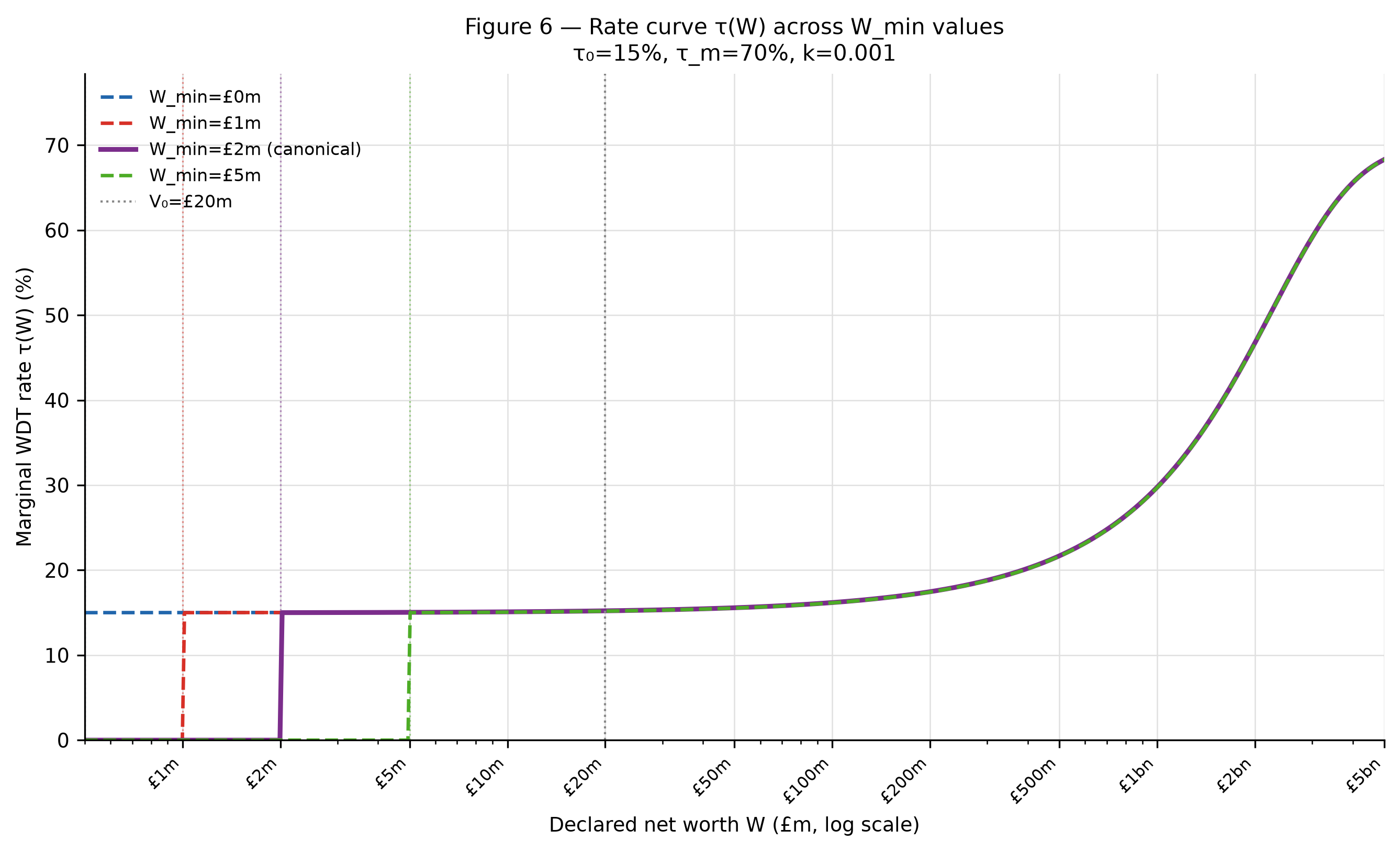
\(W_{min}\) is the wealth level below which the logistic rate function does not apply. It is the population-coverage parameter: its primary consequence is determining how many people are subject to the mechanism at all, rather than what the mechanism does to those already in scope.
6.1 What \(W_{min}\) Controls on the Declaration Mechanism (SWEEPS.V)
At \(V_0\) = £20m, \(W_{min}\) has near-zero leverage on declaration incentive properties. The C.1 heatmaps are largely stable across the four tested \(W_{min}\) values because \(V_0\) = £20m sits near the logistic floor regardless of whether the onset is at £1m or £10m — the curve’s shape above the threshold is unchanged, and the reference taxpayer’s position on it barely shifts. The N-crossing chart shows flat or gently sloping lines across \(W_{min}\) values, confirming that \(W_{min}\) has little effect on how quickly the self-limiting mechanism activates. The synthesis chart (Fig S4.3) confirms \(W_{min}\) as the parameter group with the least leverage across all three mechanism-integrity properties.
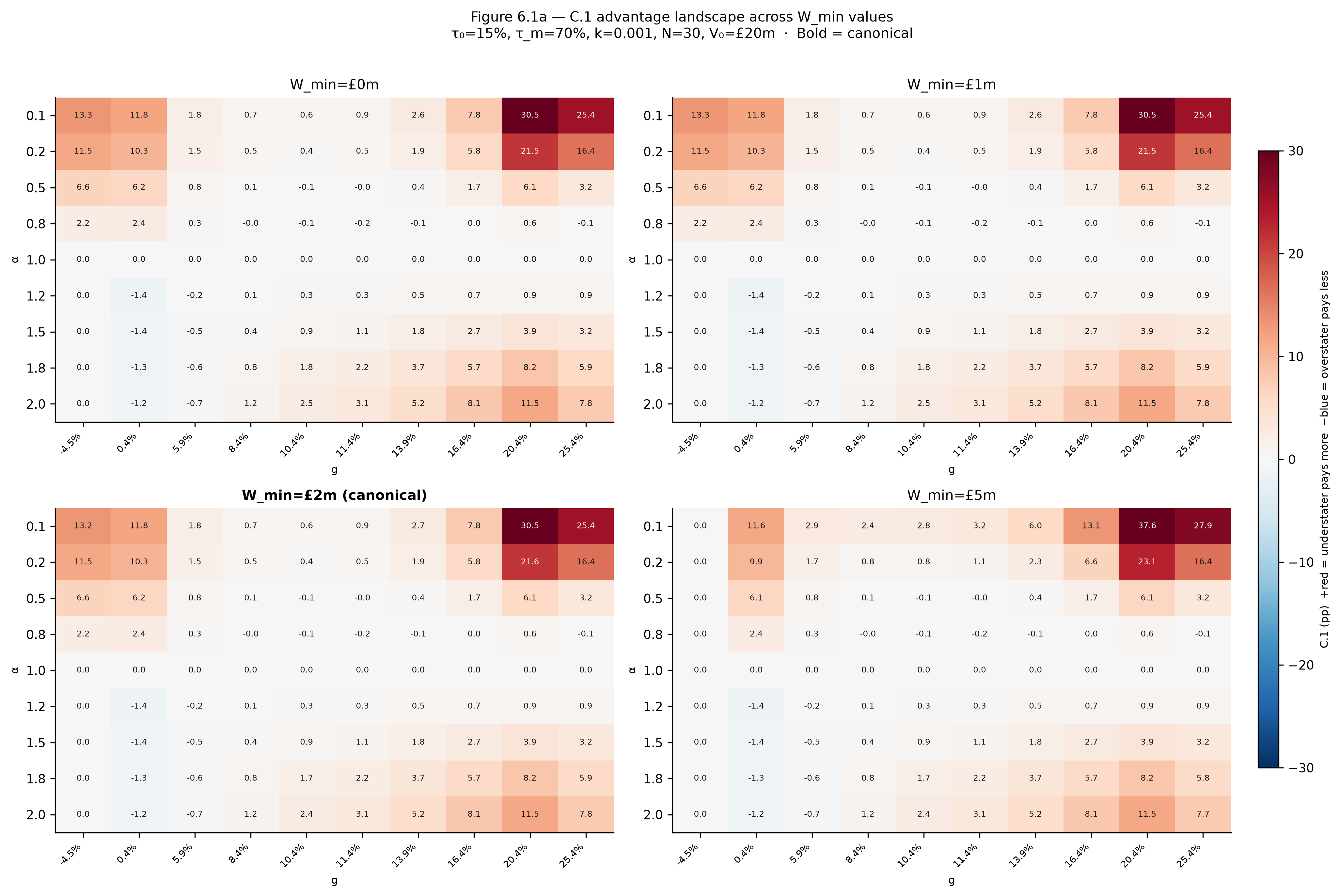
Moving \(W_{min}\) does not make the mechanism more or less forgiving, more or less deterrent, or faster or slower to self-correct for the taxpayers who remain in scope. It changes who is subject to the mechanism, not what the mechanism does to them.
6.2 What \(W_{min}\) Controls on Fiscal Outcomes (SWEEPS.R)
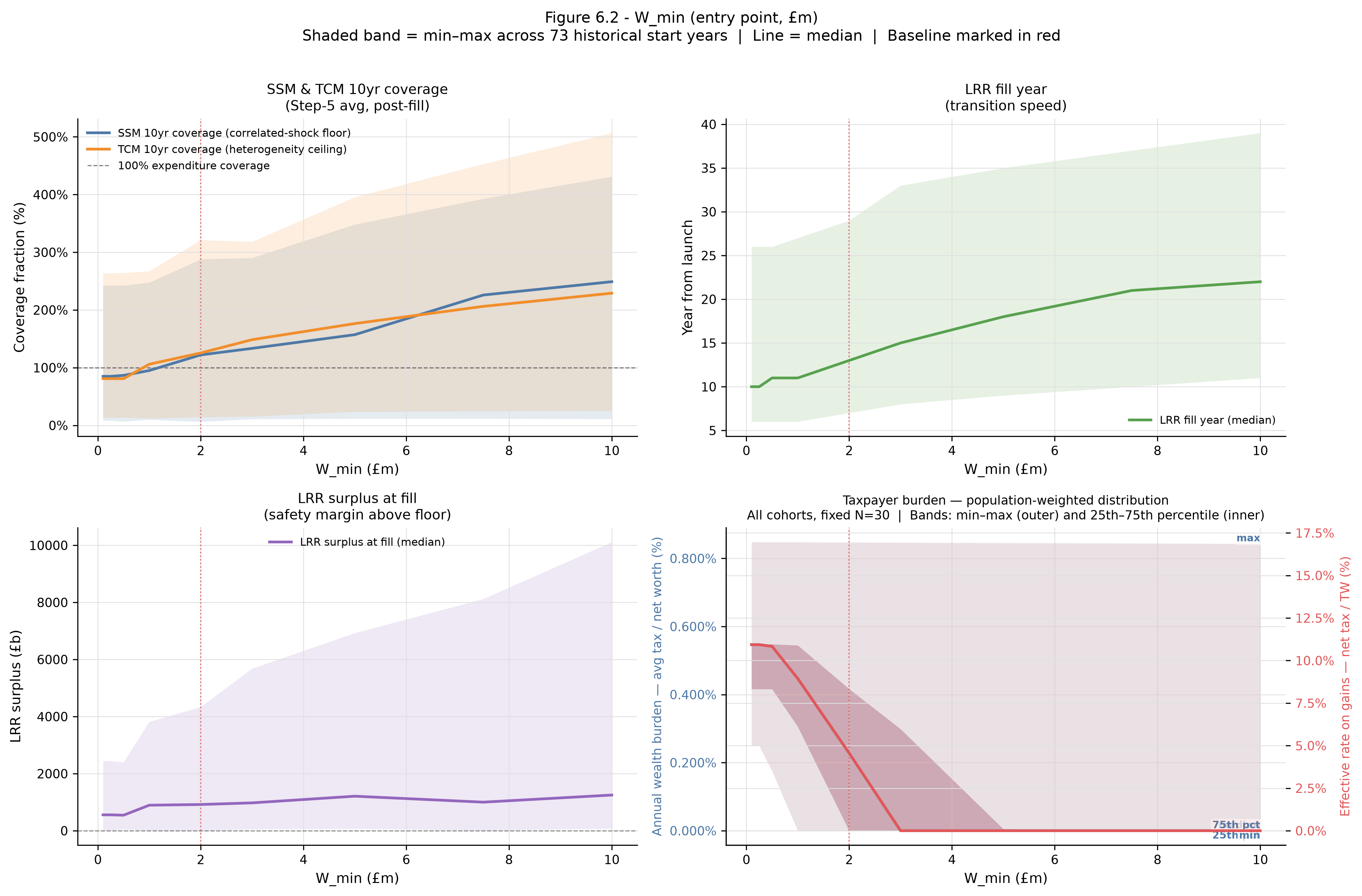
\(W_{min}\) is the second fiscal lever after \(\tau_0\) on LRR fill timing. Higher \(W_{min}\) excludes progressively more brackets from liability. Median coverage rises as \(W_{min}\) increases — at very low \(W_{min}\) (near £0m) coverage sits below 100% expenditure coverage, but as \(W_{min}\) rises and fewer lower-wealth taxpayers enter scope, coverage climbs steeply toward approximately 250% at \(W_{min}\) = £10m, driven by the denominator shift: when only upper-bracket taxpayers remain in scope, the capitalisation window opens later in the budget growth trajectory. The SSM coverage rises somewhat more slowly than TCM at high \(W_{min}\), reflecting the concentration of refund exposure onto a small high-variance taxpayer population.
The LRR fill year rises from approximately 10 years at the low end to approximately 22 years at \(W_{min}\) = £10m — the clearest structural consequence of raising the entry point: fewer taxpayers slow reserve accumulation regardless of how high the effective rates are for those who remain in scope.
6.3 What the Council Is Calibrating When It Sets \(W_{min}\)
\(W_{min}\) is the scope lever. Unlike the three rate parameters, its consequence falls almost entirely on fiscal outcomes rather than declaration incentives. A Council raising \(W_{min}\) is trading LRR fill speed for coverage and administrative simplicity: higher \(W_{min}\) slows reserve accumulation (fewer taxpayers mean less annual inflow) while simultaneously raising the coverage ratio (because the remaining population is concentrated in the upper brackets, whose per-taxpayer revenue exceeds the expenditure denominator by a larger margin). The two fiscal consequences move in opposite directions — fill timing worsens, coverage improves — and the Council’s choice about where to set \(W_{min}\) is a judgment about which dimension matters more, not a clean speed-versus-cost trade-off. Neither the declaration incentive properties nor the mechanism’s integrity for in-scope taxpayers are materially affected.
The canonical \(W_{min}\) = £2m is a judgment call rather than a threshold derived from the mechanism itself. It excludes the substantial majority of households while capturing the population where per-taxpayer revenue justifies the administrative cost. Whether the line should move is a policy question about scope and administrative economics, not a mechanism integrity question.
Chamber positions on \(W_{min}\) are less uniform than for the rate parameters, and DR’s interest is the most structurally complex. TP members near the threshold care directly; most TP members are well above any plausible \(W_{min}\) and are largely indifferent. FS cares primarily about the fiscal consequences characterised in (SWEEPS §6.2). A lottery-selected DR member’s probability of also being a WDT taxpayer depends directly on where \(W_{min}\) sits. DR members whose wealth is near or above the threshold face a split incentive: they stand to gain from labour tax relief while also facing WDT exposure, and a higher \(W_{min}\) removes the liability while preserving the dividend. DR members further from the threshold have no such tension; their primary interest is in the labour relief dividend arriving as quickly as possible, which means lower \(W_{min}\) to broaden the revenue base and accelerate LRR fill. DR’s internal division on \(W_{min}\) reflects different theories within DR about what the mechanism is ultimately for, not merely proximity to a threshold. A fuller account of how each chamber theorises its preferred parameter values across the full lever set is in (SWEEPS §6.2).
7. The Parameter Hierarchy and Its Two Faces
7.1 The Two Hierarchies
The sweep results establish two parameter hierarchies — one for fiscal outcomes, one for mechanism integrity — and on the most important single parameter they agree on direction.
The fiscal hierarchy, from SWEEPS.R: \(\tau_0\) dominates, \(W_{min}\) is second, \(k\) matters conditionally at the upper end of realistic values, and \(\tau_m\) is inert for the modelled population. The dominance of \(\tau_0\) is an artefact of canonical k: because the logistic midpoint sits at approximately £1,301m, well above the top bracket’s mean entry wealth, every bracket operates near the floor throughout the capitalisation window. \(\tau_0\) is approximately the whole rate for the modelled population. A recalibrated \(k\) that moves the midpoint into the range of the upper brackets would redistribute fiscal leverage toward \(k\) and reduce \(\tau_0\)’s dominance.
The mechanism-integrity hierarchy, from SWEEPS.V, is different in structure but not in its primary finding: \(\tau_0\) controls N-crossing timing (the overstater self-correction), \(\tau_m\) controls plateau ceiling (deterrence for egregious understaters), \(k\) controls tolerant zone width (the forgiving centre), and \(W_{min}\) has near-zero leverage on all three. A qualification on \(k\): the N-crossing panel shows \(k\) producing an 8-year range (N = 23 at \(k\) = 0.0001 to N = 15 at \(k\) = 0.005), meaning \(k\) has materially more leverage on correction timing than the primary-lever framing implies. The separability claim holds directionally, but \(k\) is not flat on the N-crossing dimension. Each parameter is doing a largely separable job. The Council can treat them as approximately independent calibration problems and use Phase One evidence on each mechanism property to revise each parameter without being forced to revisit the others simultaneously.
The key finding on \(\tau_0\) is that the two datasets agree on direction throughout the tested range. Higher \(\tau_0\) accelerates LRR capitalisation and brings the overstater correction earlier; lower \(\tau_0\) extends both. There is no \(\tau_0\) value at which fiscal capitalisation improves while the self-correction weakens, or vice versa. What \(\tau_0\) cannot do is move fiscal speed and entry burden independently: at canonical k, the floor rate is approximately what every taxpayer pays, so setting it higher means raising burden across the whole distribution. That is the concentration of consequence that makes \(\tau_0\) the most significant calibration decision the Council faces — not a conflict between the two datasets, but the fact that the parameter is doing fiscal, incentive, and political-economy work simultaneously and there is no lever that moves one without the others.
\(\tau_m\) at the canonical value is the clearest instance of complete separability: the egregious-understater deterrence lever on the declaration side, fiscally inert on the revenue side. The corrected plateau ceiling figures — approximately 37pp at canonical \(\tau_m\) = 70%, rising to approximately 65pp at \(\tau_m\) = 80% — are relevant here. The deterrence stakes of the \(\tau_m\) debate are real on the declaration side, even if the fiscal stakes are near-zero. The corrected figures make the gap between 70% and 80% clearly visible and materially larger than earlier versions of the sweep implied.
7.2 Chamber Positions and the Stabilising Effect of Disagreement
The following analysis derives the rational self-interest position of each chamber and its internal factions on each rate-function parameter. It is a theoretical exercise. Real chamber behaviour will be shaped by political conditions, social context, personal relationships, institutional culture, and behavioural factors no desk-research model can predict. Phase One is the only resolution path for those unknowns. What follows is a map of the incentive landscape, not a prediction of outcomes.
\(\tau_0\). TP has a direct financial interest in lower \(\tau_0\): at canonical k, it is approximately the whole rate they pay. TP’s position is therefore unified — lower \(\tau_0\) — with intensity scaling with wealth level. FS’s position is more complex. Higher \(\tau_0\) accelerates LRR fill and raises coverage ratios, which serves FS’s fiscal mandate; but FS also depends on DR re-election and TP political support outside the WDT, which creates pressure toward moderation. FS will not push \(\tau_0\) to its logical maximum because that risks losing TP cooperation; it will not accept TP’s preferred minimum because that extends the bootstrapping period and delays the political dividend of Phase Two. FS’s \(\tau_0\) position is a function of the political conditions of the moment — the more fiscally precarious the environment, the higher FS will push. DR is broadly aligned with higher \(\tau_0\): it accelerates both LRR fill and the overstater correction. The residual internal division is over burden — DR members who weight the mechanism’s cooperative character worry that a high entry rate signals an extractive rather than a partnership posture, which could undermine the political coalition that sustains it. The split within DR on \(\tau_0\) is less about fiscal speed versus integrity than about what entry-rate level is politically sustainable for Phase One.
\(\tau_m\). TP uniformly prefers lower \(\tau_m\): it reduces the theoretical maximum burden at extreme wealth, even though \(\tau_m\) is fiscally inert for most of the current population. The preference is symbolic as much as financial. FS uniformly prefers higher \(\tau_m\): it signals deterrence and policy seriousness at near-zero fiscal cost. DR broadly prefers higher \(\tau_m\) when the labour dividend is the salient political object, because stronger tail deterrence supports the mechanism’s long-run integrity. The \(\tau_m\) debate is the one where the fiscal stakes of the disagreement are near-zero but the symbolic stakes are high, and the chamber positions are correspondingly stable and predictable.
\(k\). TP cannot present a unified position on \(k\) because the parameter produces genuine heterogeneity of interest within the chamber. Near-threshold TP members are largely indifferent — \(k\) barely affects their bracket position. Mid-tier TP members face the sharpest rate increase from a \(k\) rise and have the strongest incentive to resist it. Ultra-HNWI TP members are already approaching \(\tau_m\) regardless of \(k\) and are relatively indifferent in the other direction. FS’s position on \(k\) depends on which fiscal argument it weights: higher \(k\) improves progressivity and concentrates consequences on very high wealth, which has political appeal; but within the current bracket structure the fiscal gain is modest. DR broadly prefers higher \(k\) insofar as stronger progressivity signals distributional intent.
\(W_{min}\). TP members near the threshold care directly; those well above it are largely indifferent. FS cares primarily about the fiscal consequences: lower \(W_{min}\) broadens the revenue base and accelerates LRR fill, moderated by administrative cost and political friction. DR is internally divided: DR members who want the labour relief dividend sooner prefer lower \(W_{min}\); DR members closer to the wealth threshold prefer higher \(W_{min}\) to keep the exemption above their own position.
The stabilising conclusion. Every rate-function parameter has at least one chamber or internal faction pulling in each direction. No parameter will be driven to its logical extreme, because every extreme position faces systematic resistance from at least one constituency with a stake in the outcome. This multi-directional pressure is an emergent property of the three-chamber structure applied to a mechanism with separable levers, not a design feature of the parameter set itself. It also means the mechanism cannot be captured by any single interest — not TP’s preference for lower rates, not FS’s preference for maximum fiscal speed, not DR’s preference for maximum redistribution pace. The separability of the levers makes capture harder: a constituency that quietly entrenches its preferred value on one parameter cannot simultaneously manipulate the others, because the parameters are observable and their effects characterised in advance. What the parameters determine is the pace and distribution of the transition, not whether it happens. The mechanism is robust to a wide range of Council-agreed values; the governance structure ensures that whatever values are agreed will be the product of genuine multi-constituency negotiation rather than any single faction’s optimum.
7.3 Growth Rate Sensitivity
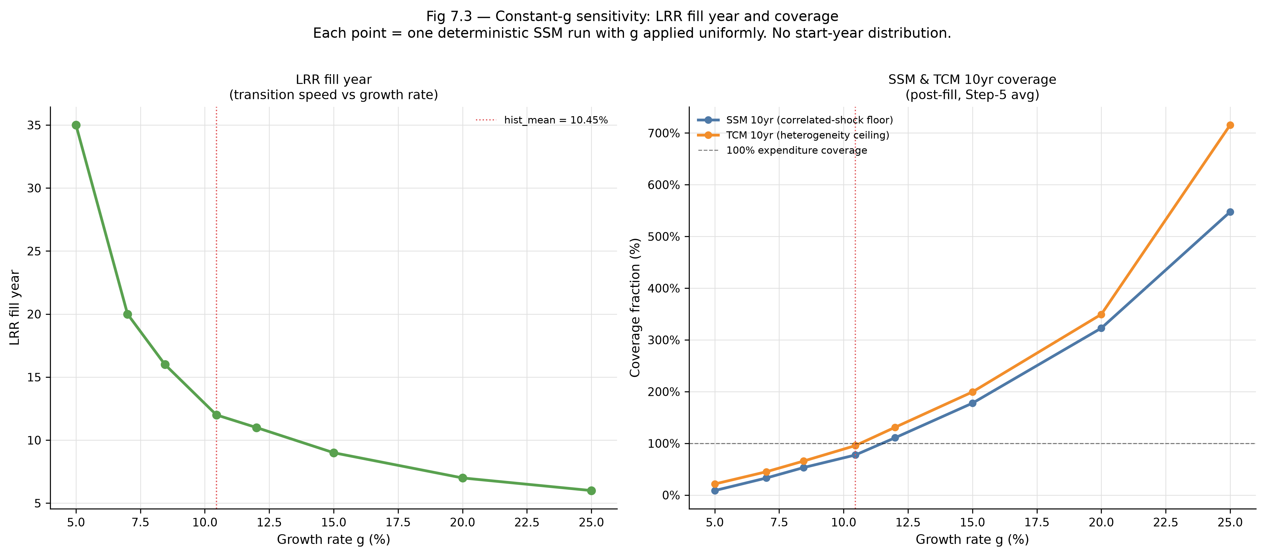
The historical sweep in (SWEEPS §7.1) applies actual UK equity return sequences and inherits whatever growth environment each start year provides. A complementary question asks what the mechanism produces under deterministic constant-growth assumptions across a range of \(g\) values — isolating the effect of the underlying growth rate from the volatility and sequencing effects that the historical return series introduces. Figure 7.3 provides this analysis.
The left panel plots LRR fill year against constant \(g\) applied uniformly to the entire taxable population through the SSM. Fill year falls steeply as \(g\) rises: at \(g\) = 5% the mechanism takes approximately 35 years to self-sufficiency; at the historical mean of 10.45% it falls to approximately 12 years; above 15% it plateaus near 6–9 years. The functional form is convex — each additional percentage point of growth reduces fill time by less than the one before it, and above the historical mean the sensitivity diminishes sharply. The steep portion of the curve lies below the historical mean, which is why the historical sweep produces such variation in LRR fill years: start years whose early periods inherit low or negative returns are effectively operating in the left tail of this curve, while boom-era starts operate near the flat portion.
The right panel plots SSM and TCM 10-year post-fill coverage against the same constant-\(g\) grid. Both series rise steeply with \(g\) and cross the 100% expenditure coverage threshold between \(g\) = 10% and \(g\) = 12% — near the historical mean. Below the historical mean the mechanism is self-sustaining but delivers sub-100% post-fill surplus in the first decade; above it the surplus compounds rapidly. At \(g\) = 25% the TCM ceiling reaches approximately 720%, which is less a forecast than a confirmation that the mechanism’s fiscal capacity scales with the wealth accumulation it taxes. The SSM and TCM series track closely at low to moderate \(g\), then diverge as persistent tier differentials compound into larger relative advantage for the higher-return tiers at elevated mean growth. The gap between the two series at high \(g\) is the within-period distributional effect of heterogeneous persistent returns: fast aggregate growth amplifies the advantage of being a Great-tier taxpayer relative to the correlated-shock baseline.
The constant-\(g\) analysis cannot substitute for the historical sweep because real return sequences are volatile, auto-correlated, and include crash years whose sequencing matters for SRR and LRR dynamics. What it contributes is legibility: a single curve the Council can use to locate any given growth environment on the fill-time and coverage scales, and to read off the rough implications of sustained growth environments materially above or below the historical mean.
7.4 Cross-Parameter Coverage Fan
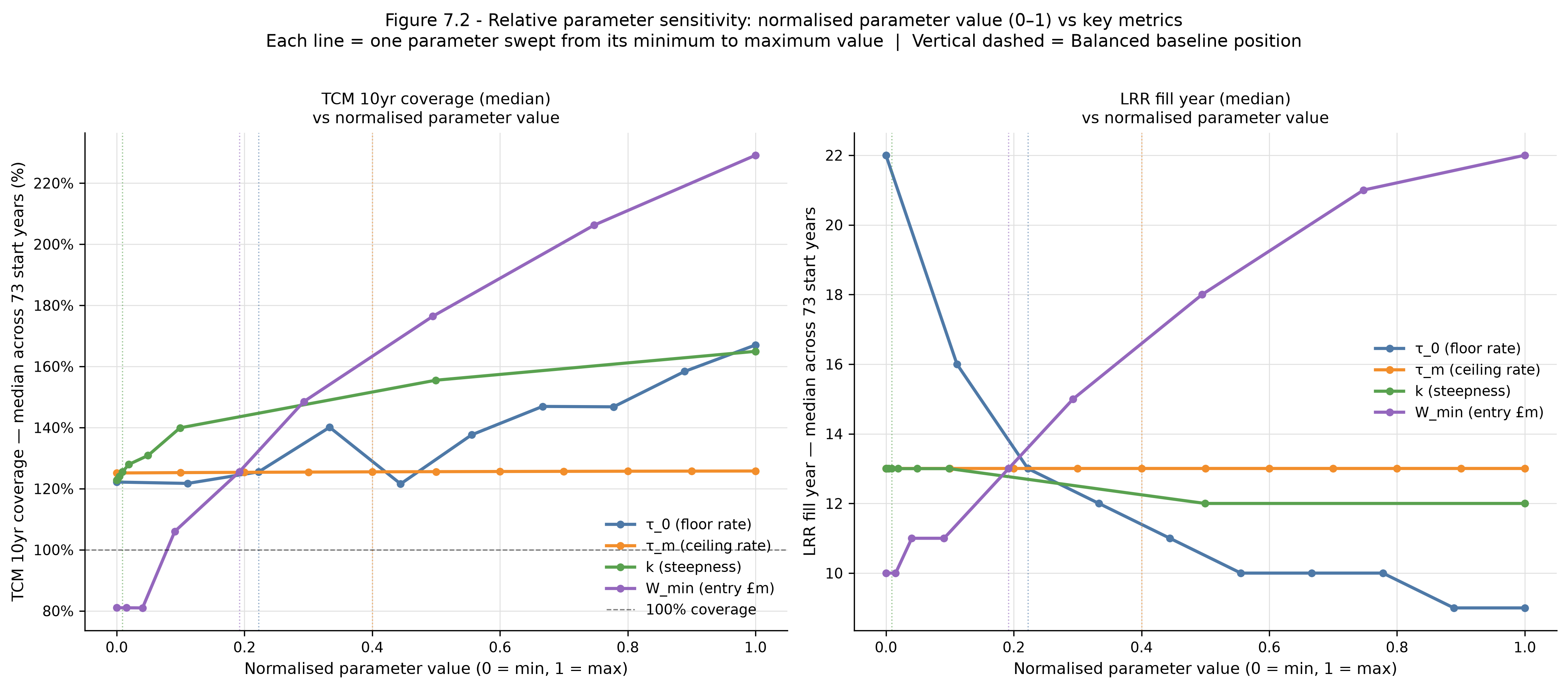
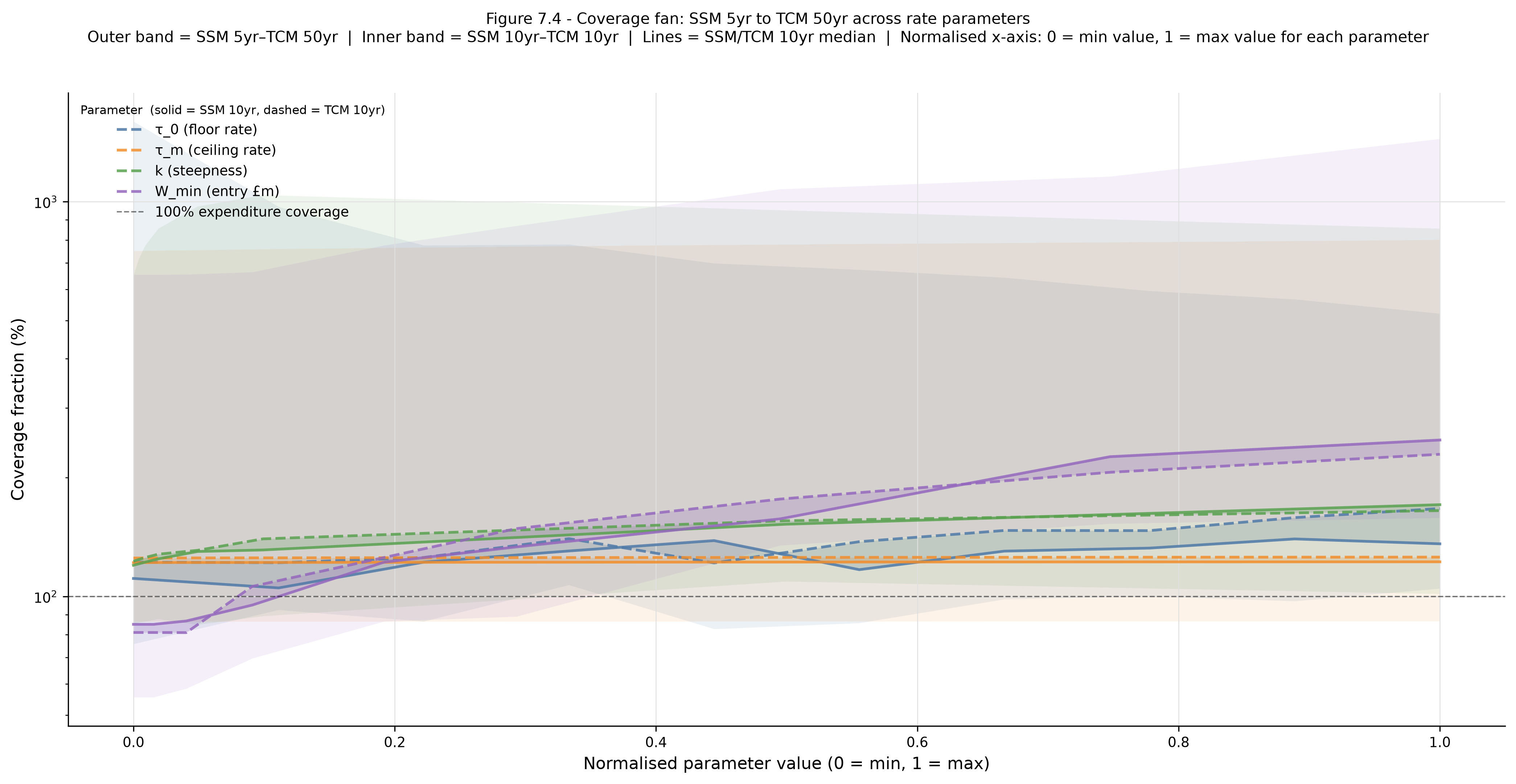
Figures 7.1 and 7.2 present each parameter’s fiscal consequences on separate panels. Figure 7.4 overlays all four parameters on a single log-scale chart, plotting coverage as a function of normalised parameter value (0 = minimum tested, 1 = maximum tested). This makes the relative steepness and direction of each parameter’s fiscal leverage directly comparable.
Three properties are immediately visible. First, \(\tau_m\) (orange) is flat at approximately 130% median SSM/TCM 10yr coverage throughout its full normalised range — the fiscal inertness established in (SWEEPS §4.2) is visible as a horizontal line against which all other parameters can be calibrated. Second, \(\tau_0\) (blue) and \(k\) (green) both rise with their parameter value, but \(\tau_0\)’s slope is steeper and more monotone: \(\tau_0\) is the dominant fiscal lever, consistent with the hierarchy in (SWEEPS §7.1). Third, \(W_{min}\) (purple) begins below 100% at its minimum value (very low threshold, many low-wealth taxpayers generating modest aggregate revenue relative to expenditure) and rises steeply through 100% as the threshold increases and the taxable population concentrates in higher-revenue brackets. The purple line crosses the 100% reference at roughly the midpoint of its range, confirming that canonical \(W_{min}\) = £2m sits in the moderate-coverage portion of the feasible scope.
The shaded bands show the SSM 5yr–TCM 50yr range — the widest bracket of coverage outcomes across both models and window lengths. These bands are wide because they span both the lowest-coverage short windows and the highest-coverage long windows, and because the SSM/TCM distinction compounds the window-length difference. The inner bands (SSM 10yr to TCM 10yr) are the relevant comparison for the 10-year post-fill metric used throughout this paper. The outer bands confirm that the mechanism never produces coverage below approximately 30% of expenditure at any tested parameter value across any coverage window — a robustness floor that is visible directly in the chart.
7.5 Synthetic Stress-Test: Cyclical Growth Scenarios
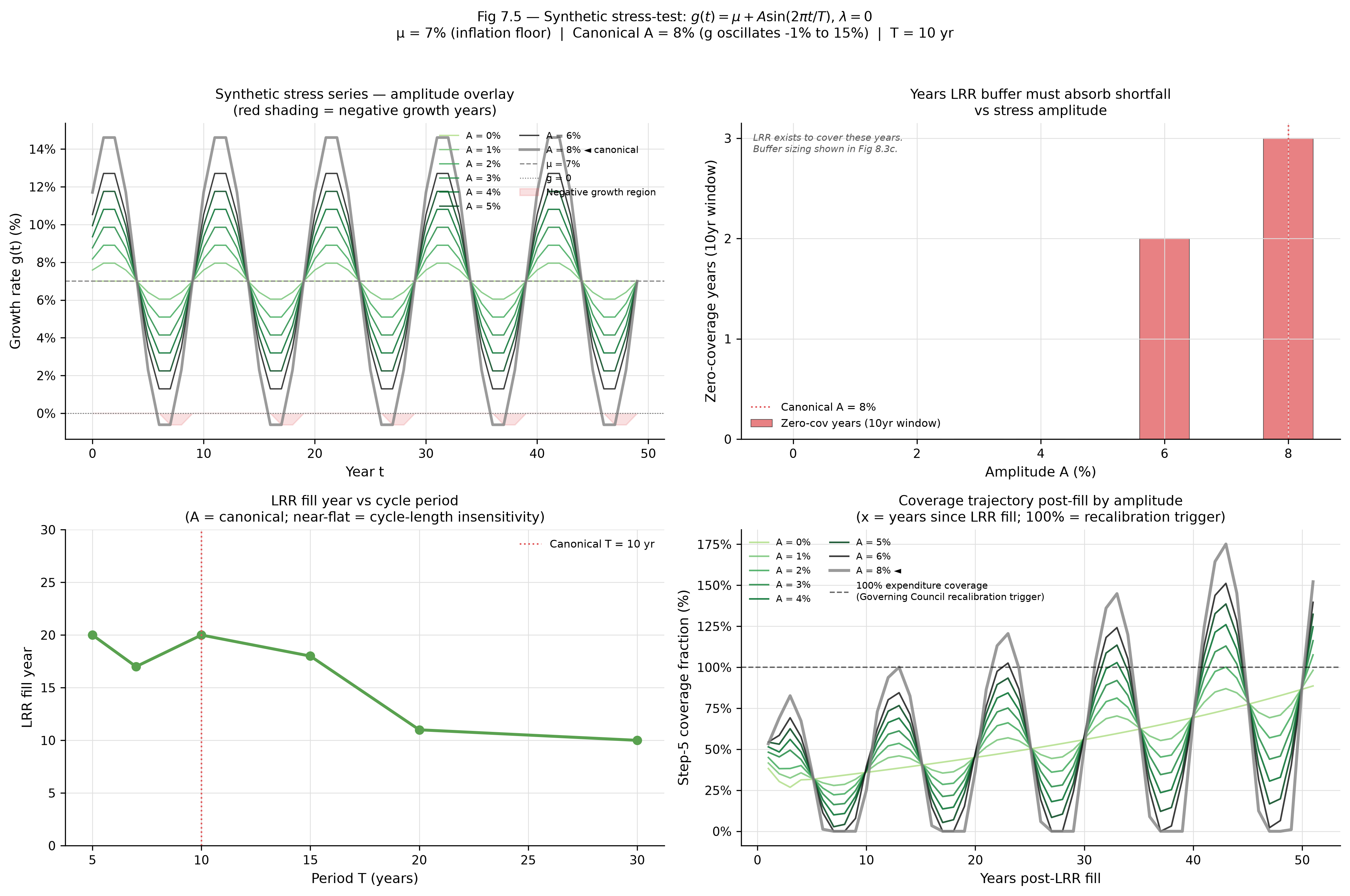
The historical sweep applies real UK equity return sequences. The constant-\(g\) analysis applies uniform deterministic growth. A third mode of investigation applies a stylised sinusoidal growth trajectory of the form \(g(t) = \mu + A\sin(2\pi t / T)\), where \(\mu\) is the mean return, \(A\) is the amplitude of the cycle, and \(T\) is the period. This synthetic stress-test isolates the effect of cyclical volatility independently of the sequencing and distributional properties that make historical return series difficult to interpret in isolation.
The canonical specification uses \(\mu\) = 7% (approximately inflation floor for real asset appreciation), \(T\) = 10 years (one decade per full cycle), and a central amplitude of \(A\) = 8%, which produces growth oscillating between approximately −1% and +15%. At this amplitude the model experiences negative growth years (red-shaded troughs in the top-left panel of Figure 7.5), triggering the symmetric refund mechanism and drawing on the SRR in those years.
Four results emerge from the sweep across amplitude \(A\) and cycle period \(T\).
First, the mechanism handles moderate cyclical volatility without accumulating deficit. For amplitudes \(A\) ≤ 5% the zero-coverage year count in the 10-year post-fill window is zero — every year delivers positive Step-5 surplus and the LRR is never drawn below floor. Negative growth years still occur at the canonical \(A\) = 8%, but the refund flows they generate are absorbed by the SRR rather than the LRR, and the LRR recovers in subsequent positive-growth years. Two zero-coverage years appear in the 10-year window at \(A\) = 6%, rising to three at the canonical \(A\) = 8% — the same order of magnitude as the historical sweep’s worst-case start years.
Second, LRR fill year is largely insensitive to cycle period \(T\) once \(T\) is above approximately 7 years. The bottom-left panel shows fill year near 20 years at \(T\) = 10 (the canonical), falling to approximately 11 years at \(T\) = 30, with non-monotone behaviour below \(T\) = 7. The near-flat region above \(T\) = 10 confirms that the fill dynamics are primarily determined by the mean return \(\mu\) rather than the cycle period — consistent with the constant-\(g\) finding that mean growth is the dominant driver of transition speed.
Third, the coverage trajectory post-fill oscillates with the cycle but never collapses. The bottom-right panel shows Step-5 coverage fraction by year since LRR fill for each amplitude level. All series oscillate around a rising trend; the 100% reference line (the Governing Council recalibration trigger) is crossed periodically even at the canonical \(A\) = 8% amplitude. This is the correct response: the governance architecture’s mandatory rate review mechanism (GOV §6) is designed to fire when the Step-5 surplus consistently exceeds 100% of expenditure, redirecting surplus toward the labour tax relief dividend rather than accumulating further in the LRR. The oscillating coverage trajectory is the mechanism behaving as intended, not a solvency concern.
Fourth, the zero-coverage year count is small and bounded at realistic amplitudes. Three zero-coverage years in a 10-year post-fill window means the LRR covers three years of expenditure shortfall — precisely the purpose of a 3× LRR floor. The synthetic stress-test confirms that the buffer sizing in (SWEEPS §8.3) is calibrated against the right order of cyclical stress.
8. The Operational Parameters
The rate-function parameters are the primary subject of this paper. The operational parameters below complete the lever inventory but receive shorter treatment: sweep data does not yet exist for most of them, and their calibration is more dependent on Phase One evidence than on prior characterisation.
8.2 The \(\tau_{h}\) Ramp
The \(\tau_{h}\) ramp governs how quickly the final charge on permanently unattributable corporate ownership rises toward its ceiling. It cannot be calibrated in isolation: as established in (CORP.A §B.2), the ramp must be co-designed with the CIT and dividend displacement schedule as a joint trajectory. TP is internally divided along industry lines — TP members from transparent-ownership structures favour faster progression; those from attribution-hard industries have an incentive to reveal the actual constraints on attribution feasibility accurately, which gives the Allocator’s inside knowledge particular value here. FS wants fast progression for attribution coverage. The joint-calibration constraint limits what any single chamber can unilaterally push for, since moving \(\tau_{h}\) without moving CIT and dividend displacement creates a wedge that advantages opacity as a hedge.
8.3 The LRR Drawdown Pace
The LRR drawdown pace determines how quickly the LRR disburses once the floor is met. Chamber alignment here is closer to uniform than for any rate-function parameter: DR wants faster disbursement, FS wants to demonstrate delivery, and most TP members are broadly supportive. The corrective is the subset of TP with large volatile portfolios who have a financial interest in SRR adequacy — drawdown acceleration that threatens the SRR buffer is not in their interest. This corrective is real but contingent on TP composition at any given moment; the Custodian’s actuarial mandate is the non-contingent institutional safeguard.
Calibration of drawdown pace is highly sensitive to Phase One findings. The SRR and LRR floor targets — set at 3× net annual WDT income and 3 years of government expenditure respectively — are judgment calls, but (SWEEPS.A §C.6) to (SWEEPS.A §C.7) now characterises their sensitivity across the full 73-year historical sweep. The srr_ratio sweep shows 100% success across all tested values (1× to 10×); the 3× recommended floor is the threshold below which the 2006 worst-case scenario first shows an SRR breach (covered by the LRR balance at 1×, 1.5×, and 2×; breach-free from 2.5× onward), confirming the floor is appropriately placed rather than systematically conservative. The lrr_years sweep shows LRR fill year scaling directly with the floor target (median 6yr at 0.5 years, 24yr at 8 years) with 100% success throughout; the 3× floor gives the canonical median of 13yr. The SRR fill year rises one-for-one with srr_ratio and is otherwise invariant. What neither sweep can provide is the empirical test of solvency behaviour under an actual downturn; Phase One data on that remains the input that would allow confirmation or revision of both floors.
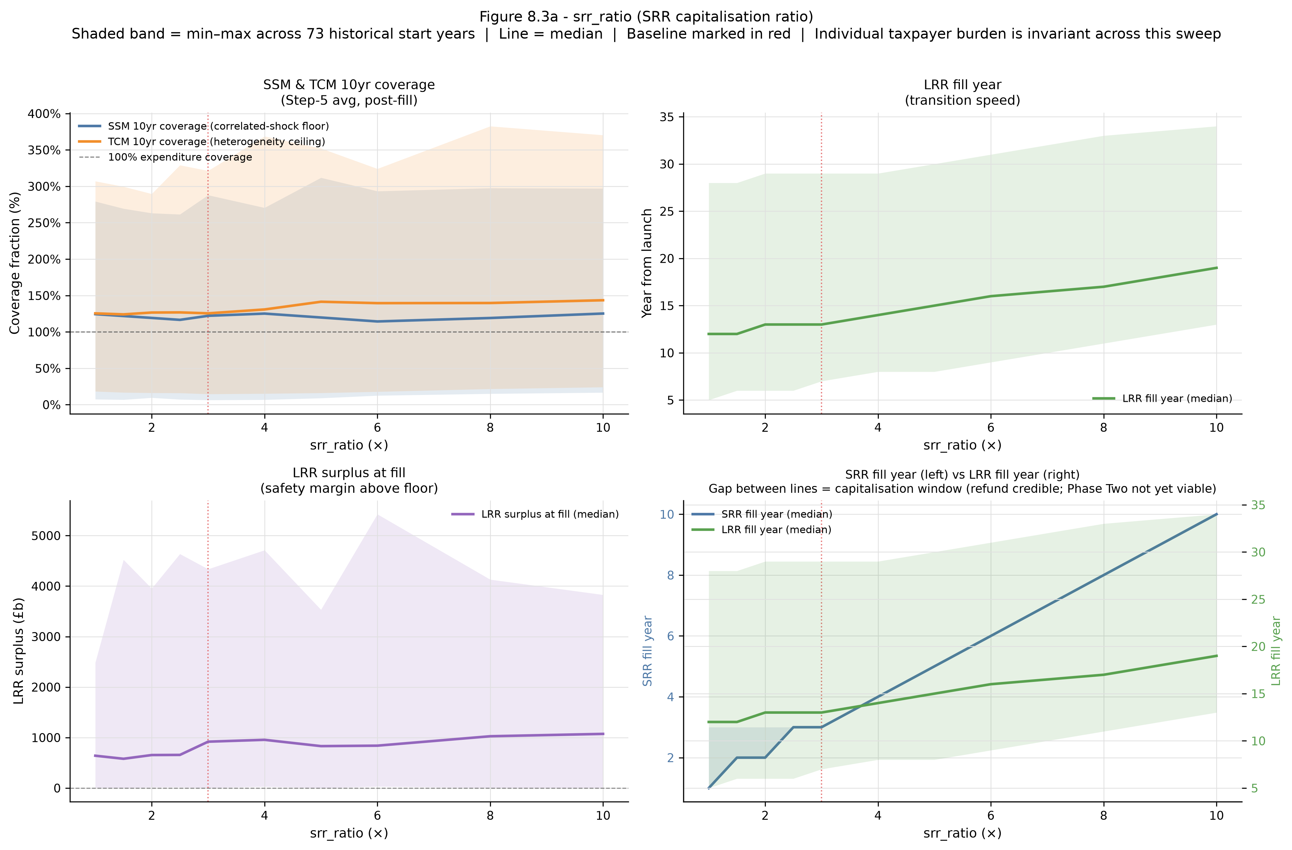
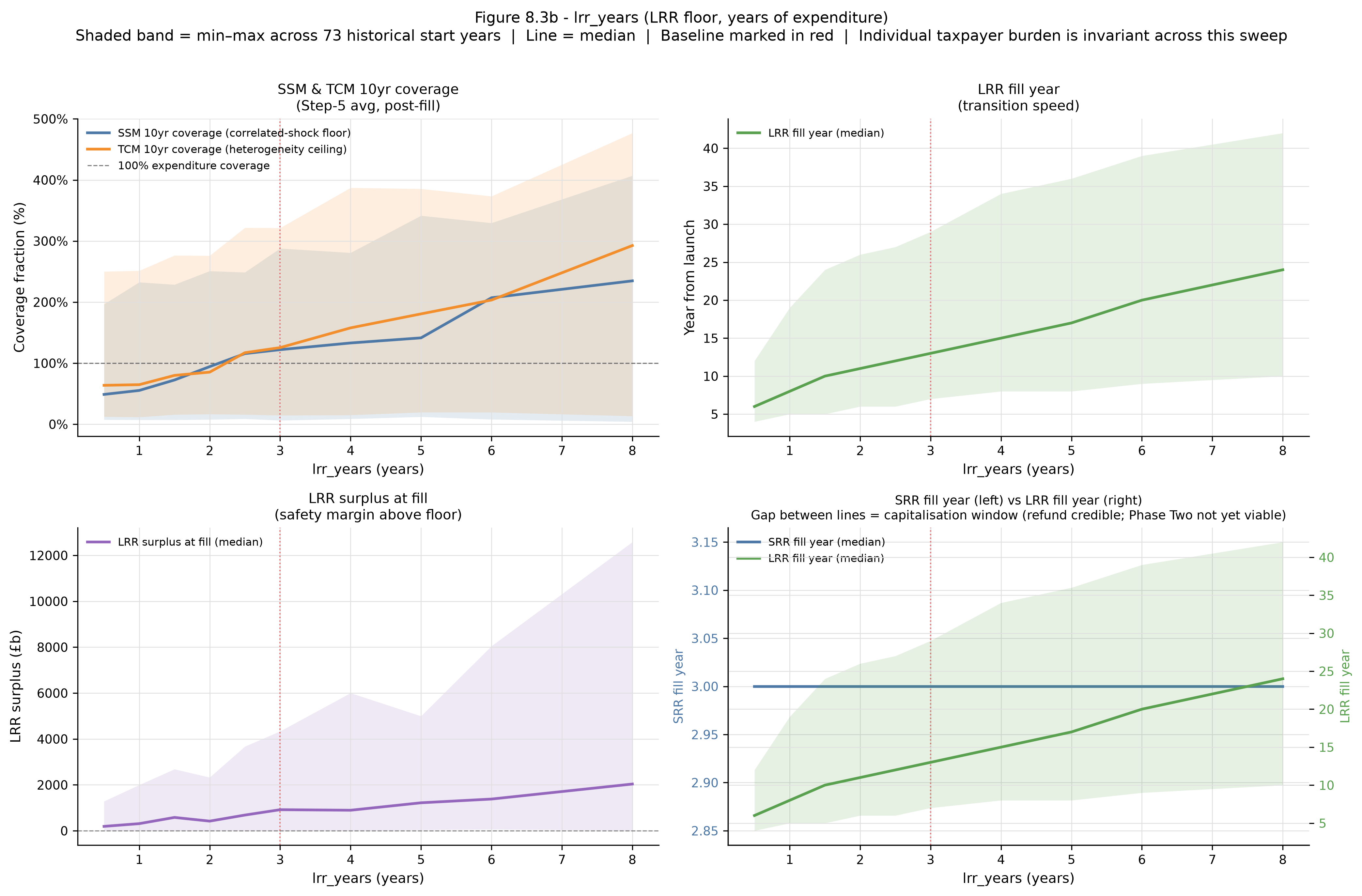
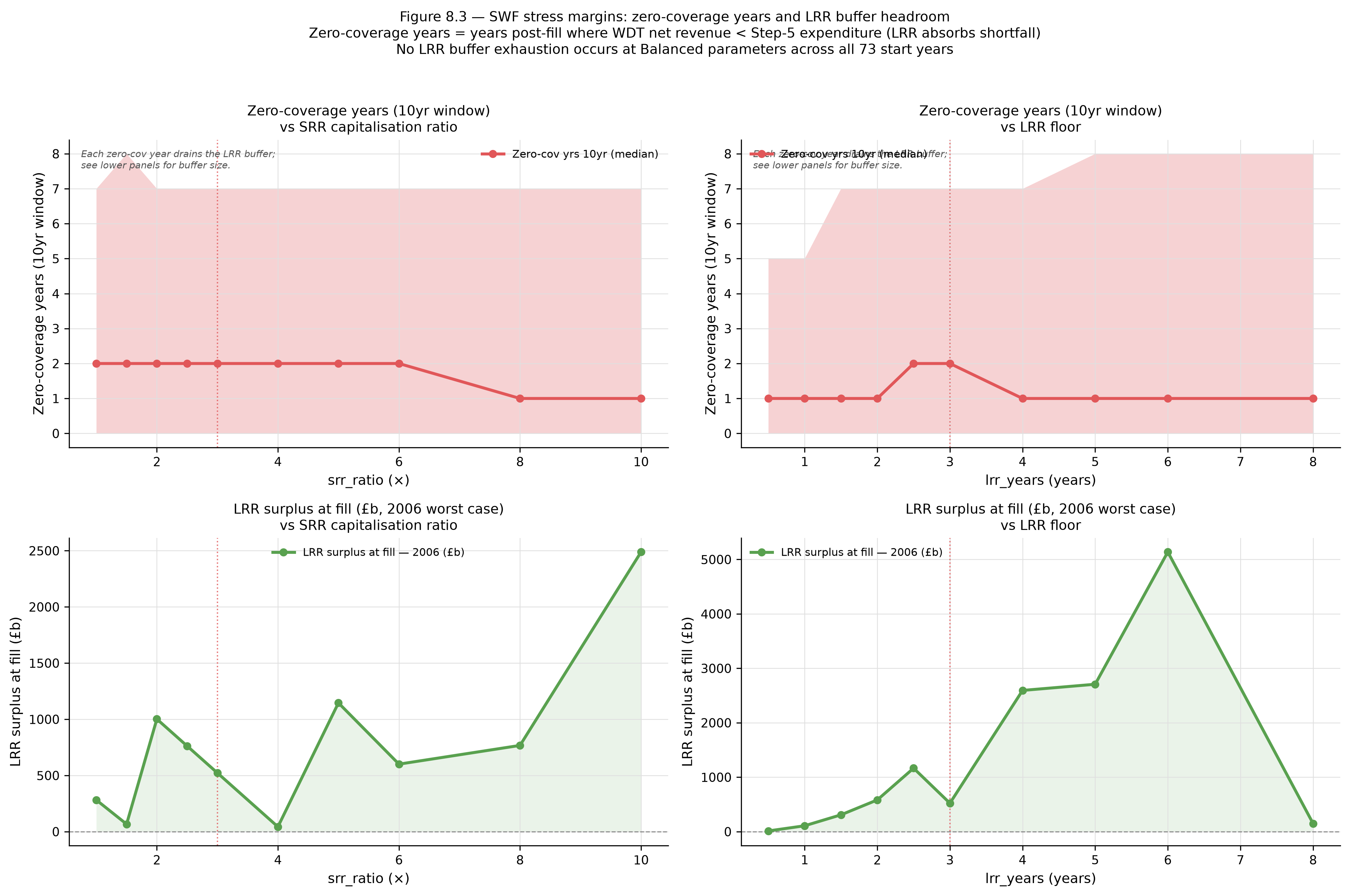
Figures 8.3a and 8.3b establish how srr_ratio and lrr_years affect fill timing and surplus at fill. Figure 8.3c adds the stress margin perspective: how many zero-coverage years the mechanism encounters in the 10-year post-fill window, and how much LRR buffer headroom remains at fill in the worst historical start year (2006). These two quantities determine the practical adequacy of each floor setting, independent of the fill timing dimension.
Zero-coverage years are years where WDT net revenue falls below the Step-5 expenditure target — years the LRR must absorb rather than contribute. Each zero-coverage year drains the LRR buffer; the buffer must be large enough to absorb the cumulative drain across a realistic run of such years. The top panels show that the zero-coverage year count is stable at 1–2 years across the srr_ratio sweep (top-left) and varies between 1 and 2 years across the lrr_years sweep at canonical lrr_years = 3, with a transient elevation near lrr_years = 2.5 (top-right). These figures are medians across all 73 start years; the shaded bands show the range.
The LRR surplus at fill (bottom panels) shows the headroom available in the 2006 worst-case scenario — the start year that produces the slowest LRR fill and therefore the thinnest surplus. At the canonical srr_ratio = 3×, the 2006 surplus at fill is approximately £523b (consistent with the extremal cases table in SWEEPS §7.1). The surplus rises irregularly with srr_ratio, reaching approximately £2,500b at srr_ratio = 10×, but the relationship is non-monotone — the surplus reflects where in the return sequence the extended capitalisation window terminates rather than a simple scaling of the floor. Across the lrr_years sweep the canonical 3-year floor delivers approximately £523b of 2006 surplus at fill; the relationship rises to peaks near lrr_years = 5–6 years before compressing back at 8 years.
The practical implication: the canonical srr_ratio = 3× and lrr_years = 3 settings deliver 1–2 zero-coverage years in the median post-fill decade and approximately £523b of LRR buffer in the worst historical start scenario — enough headroom for several years of full LRR drawdown at prevailing expenditure levels. The floor settings are appropriate; raising either does not improve the zero-coverage year count materially while substantially extending the fill timeline.
8.4 Route C Rotation Pace
The Route C rotation pace determines how quickly the SWF rotates equity positions acquired through in-kind settlement into its standard asset allocation. Under inflationary conditions the trigger threshold for accelerated rotation is a Governing Council parameter (GOV.B §E.7); the automaticity of the rotation itself is built into the Custodian’s mandate, but the threshold that activates it is not. FS prefers a lower trigger threshold — faster rotation provides countercyclical inflation response sooner. TP is divided: those with large Route C positions prefer slower rotation to avoid forced market timing; those without are largely indifferent. DR broadly supports faster rotation insofar as it protects the real value of the LRR.
8.5 The Privacy Rate Differential
The privacy rate differential — the rate premium on undisclosed assets and discount on disclosed ones — affects two things simultaneously: declared-value quality and SRR exposure. Higher differential improves declaration transparency, which benefits the public register and the mechanism’s audit capacity; it also increases the SRR’s sensitivity to the distribution of privacy elections across the taxable population, since refunds in loss years are calculated on declared bases. TP prefers lower differential to preserve optionality; FS prefers higher to improve attribution coverage; DR broadly supports higher insofar as transparency strengthens long-run mechanism legitimacy. The parameter is a single coefficient whose revenue neutrality in expectation is a constraint (GOV.B §B.4.7) rather than an outcome to optimise.
8.6 Corporate Facility Parameters
The corporate equity settlement facility parameters — loan rate, repayment schedule, margin call threshold, and maximum holding period — are largely technocratic calibrations informed by the Custodian’s portfolio risk assessment and Phase One take-up data. If the corporate attribution mechanism functions as designed, unattributed ownership approaches zero and the facility’s revenue contribution is negligible. The realistic expectation is that attribution will be imperfect, the facility will carry some permanent load, and Phase One data on take-up rates and repayment behaviour will be the primary input to any calibration revision. Cross-reference: (CORP §6) and (RATES §5.2)
9. The Small Lever Set as a Design Feature
The preceding sections are descriptive. This section makes a normative argument. The WDT’s small lever set is not a constraint on fine-tuning — it is a deliberate architectural choice with consequences for democratic accountability that are independent of whether the parameters land at any particular value.
Current tax systems accumulate parameters across decades of incremental legislation. Rate schedules interact with reliefs, which interact with thresholds, which interact with timing rules, which interact with entity classifications. Even informed practitioners cannot reliably predict the effect of changing any single element in isolation, because the interactions are too numerous and too path-dependent to trace cleanly. This opacity is not incidental — it is the medium through which capture operates. A parameter whose effect cannot be characterised cannot be held accountable.
The WDT’s four rate-function parameters are doing largely separable jobs, as (SWEEPS §3) to (SWEEPS §6) establish. The Council can know, in advance, what adjusting each lever will do — to revenue, to declaration incentives, and to the balance between them. A vote on \(\tau_0\) has characterised consequences that any motivated observer can track and evaluate against the outcome. A vote on \(\tau_m\) has near-zero fiscal consequence and well-defined tail-deterrence consequences. A vote on \(k\) moves the progressivity of the rate schedule in a direction that can be stated and verified. A vote on \(W_{min}\) changes the scope of the mechanism in a way that is directly observable in the number of taxpayers assessed. None of these is opaque.
The optimality cost of a small lever set is real and should be stated plainly. There will be cases where the right answer requires a combination of adjustments the mechanism cannot accommodate without cross-parameter consequences. The most visible current case is \(\tau_0\): no single setting simultaneously sets the entry burden low, fills the LRR quickly, and brings the self-correction earliest. All three dimensions move together with \(\tau_0\), which means the Council cannot optimise each independently — it must choose a level and accept the package. That is a constraint, not a failure of mechanism design. The mechanism does not eliminate these trade-offs; it makes them legible. A vote on \(\tau_0\) is a single observable decision with characterised consequences across three dimensions. That is a different and more modest claim than optimality, but it is the correct one.
Phase One is where this argument is put to the test. A small lever set generates cleaner evidence about what each adjustment does precisely because the parameters are separable. When the Council adjusts \(\tau_0\) in response to Phase One declaration data, the effect on fiscal outcomes can be isolated from the effect of any simultaneous \(k\) or \(W_{min}\) movement, because the parameters are not deeply entangled. A Council completing Phase One with interpretable evidence on each mechanism property will be better positioned to make informed calibration decisions than any pre-implementation body could be, not because Phase One proves the mechanism works, but because the evidence it generates is readable. A system with dozens of interacting parameters generates confounded evidence; a system with four separable ones generates evidence that points somewhere.
10. What Phase One Needs to Measure for Calibration
For each rate-function parameter, the following identifies the Phase One data that would allow the Council to refine its position. This section does not specify evaluation designs — those are in (PHASE1 §5) — but records what each parameter is waiting for.
\(\tau_0\). The primary signal is declared value distributions relative to subsequent realisation prices. If the lower tolerant-zone boundary is set too low — meaning mild understatement is cheaper than the mechanism intends — the signal appears as systematic understatement just below the threshold, visible in the gap between declared values and realised prices at sale. If the entry rate is producing stronger behavioural response than expected — whether faster convergence of declared and realised values, or evidence of avoidance restructuring — that is the signal that the \(\tau_0\) level is exerting meaningful pressure on declaration behaviour, and the Council can use that evidence to assess whether the current balance between pace and cooperative posture is well-calibrated.
\(\tau_m\). The primary signal is loss-year refund claims relative to prior-year contribution histories. Egregious understatement at high growth rates should produce large refund claims in loss years from taxpayers with large prior contribution histories — the plateau ceiling is doing its work. If refund claims in the first significant downturn are systematically lower than the plateau ceiling predicts, \(\tau_m\) may need upward revision; if the refund exposure is larger than the SRR floor can comfortably absorb, the relationship between \(\tau_m\) and the SRR multiplier requires joint review.
k. The primary signal is the distribution of declared net worth across the taxable population — specifically, where most taxpayers sit on the rate curve. If the bulk of revenue-generating taxpayers cluster in the near-flat portion of the logistic throughout Phase One, \(k\) is functioning as intended at canonical values. If declared wealth is concentrated at levels where the curve is already steep, \(k\) may be more consequential than the current sweep data suggests, and the fiscal hierarchy in (SWEEPS §7.1) would need revision.
\(W_{min}\). The primary signal is the distribution of near-threshold taxpayers across the exemption boundary, together with administrative cost per taxpayer at different wealth levels. Whether the £2m canonical threshold is set too high or too low is not determinable before Phase One.
LRR drawdown pace and the reserve multipliers. The primary signal is SRR behaviour under the first significant market downturn. The current 3× SRR and 3× LRR floor multipliers are judgment calls; Phase One downturn data is the empirical input that would allow either revision or confirmation. The Custodian’s actuarial mandate is the interim safeguard until that data exists.
11. Limitations
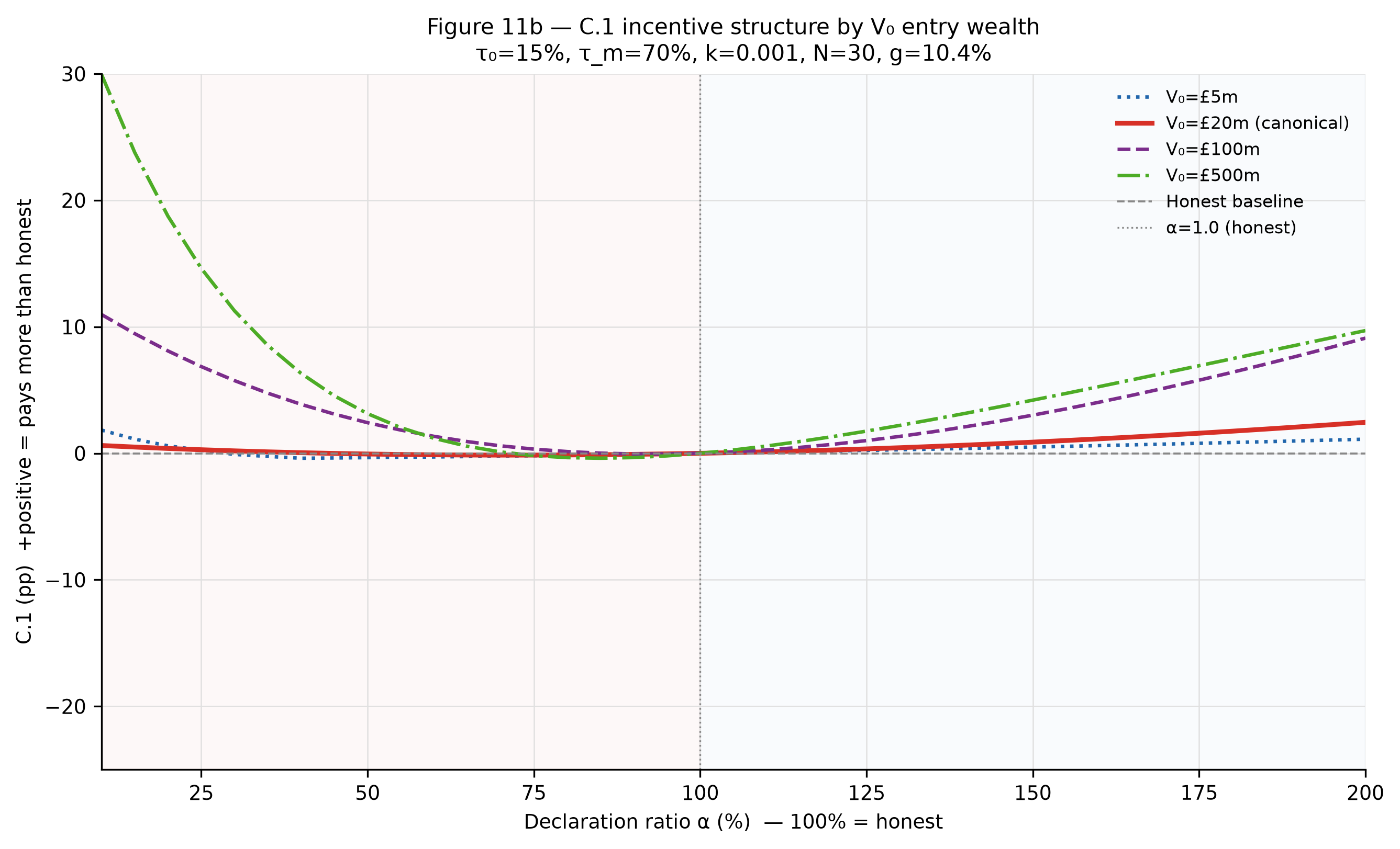
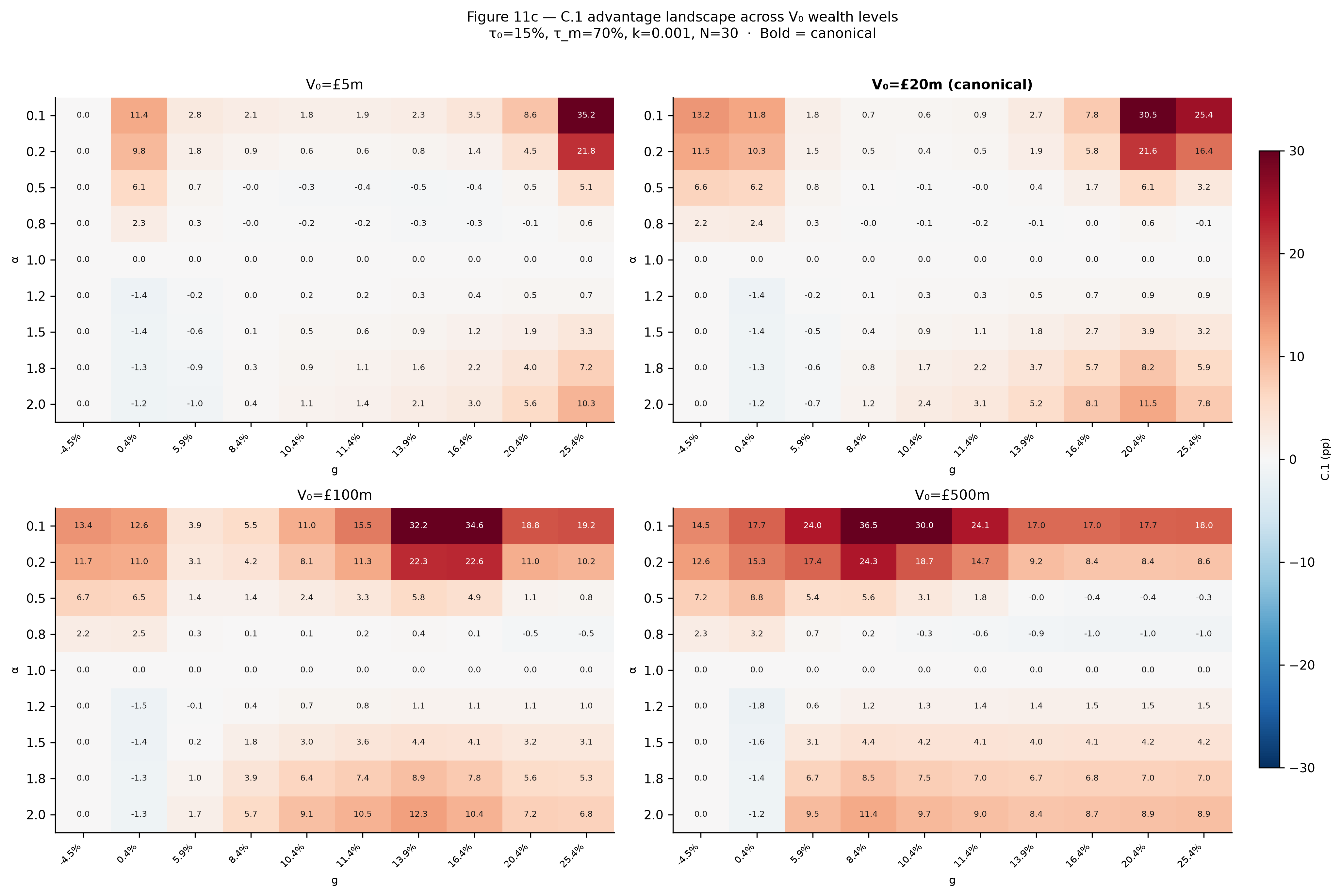
Population-level extrapolation. SWEEPS.V uses a single reference taxpayer at \(V_0\) = £20m. Mechanism properties vary materially with entry wealth — the C.1 landscape at \(V_0\) = £500m differs substantially from the canonical reference, with understater penalties and overstater correction magnitudes both intensifying significantly at higher wealth. The chamber theory in (SWEEPS §7.2) and the Phase One measurement programme in (SWEEPS §10) both implicitly assume that the \(V_0\) = £20m reference is representative of the declaration incentive structure across the taxable population. It is not. The\(V_0\) sweep (§B.5) shows that near-threshold taxpayers face correction magnitudes of approximately 1–2pp at N = 30, while taxpayers at £500m face correction magnitudes of approximately 8–10pp. A full population-weighted analysis requires distributional assumptions about \(V_0\) that are not available before Phase One, and the single-reference-taxpayer results should be read as indicative of mechanism direction rather than quantitatively accurate for the population as a whole. Importantly, this limitation cuts in a direction that is conservative for the mechanism’s robustness claims: the canonical reference understates mechanism intensity for precisely the taxpayers who generate most WDT revenue. The self-correction and deterrence properties shown at \(V_0\) = £20m are weaker than those the mechanism actually produces at the wealth levels that matter most fiscally.
Constant growth assumption. The N-crossing analysis assumes constant \(g\) across all years in the system. Real portfolio trajectories are volatile: a taxpayer whose wealth underperforms early and outperforms late faces a different correction profile than the constant-g model, and vice versa. The N-crossing threshold is better understood as an expected-value result under constant growth rather than a prediction of when any individual taxpayer will encounter the correction. This limitation is inherited from VAL.A and repeated here because the N-crossing figures are load-bearing in the parameter hierarchy analysis of (SWEEPS §7.1).
Revenue sweep partially complete. The rate-function sweeps (\(\tau_0\), \(\tau_m\), k, \(W_{min}\)) and reserve-multiplier sweeps (srr_ratio, lrr_years) are confirmed in SWEEPS.A. What remains open is the interaction surface: the \(\tau_0\) × \(W_{min}\) joint sweep, which would quantify the primary cross-dataset tension across the joint parameter space rather than characterising it from single-parameter-at-a-time results. The full quantification of revenue sensitivity interactions is the natural RATES.A extension. The parameter hierarchy in (SWEEPS §7.1) should be read as provisional pending that work, particularly the dominance of \(\tau_0\), which is an artefact of canonical \(k\) rather than an architectural property.
Reserve multiplier sweeps confirmed. (SWEEPS.A §C.6) to (SWEEPS.A §C.7) sweep srr_ratio (1× to 10×) and lrr_years (0.5 to 8 years) independently across all 73 historical start years. Both achieve 100% success throughout. The 3× srr_ratio floor is confirmed as appropriately placed: the 2006 scenario shows covered SRR breach below 2.5× and no breach from 2.5× onward. The lrr_years sweep confirms the 3× floor gives a canonical median fill of 13yr. The residual — empirical confirmation of solvency behaviour under an actual downturn — is a Phase One item and cannot be resolved by historical simulation.
SWEEPS.V figures confirmed. All quantitative values cited in (SWEEPS §3) to (SWEEPS §6) are drawn from SWEEPS.A, generated at confirmed canonical parameters (\(\tau_0\) = 15%, \(\tau_m\) = 70%, \(k\) = 0.001, \(W_{min}\) = £2m, N = 30). N-crossing thresholds, plateau ceiling magnitudes, and fiscal coverage ranges reflect those confirmed tables.
k sweep confirmed. The \(k\) sweep in SWEEPS.A (A.3 and B.4) was run across nine log-spaced values from \(k\) = 0.0001 to \(k\) = 0.1 at confirmed canonical (SWEEPS §5) reflects those results. The \(\tau_m\) fiscal inertness finding in (SWEEPS §4.2) and the logistic midpoint characterisation in (SWEEPS §5.3) both stand at canonical \(k\) = 0.001: the top bracket reaches mean wealth of approximately £1,266m at year 30, which sits well below the midpoint of approximately £1,301m, and no bracket approaches the ceiling rate during the capitalisation window.
Joint surfaces limited. The interaction analysis covers \(\tau_0\) × N and \(k\) × \(V_0\) only. The \(\tau_0\) × \(W_{min}\) joint surface would quantify how the two primary fiscal levers interact across their joint parameter space — currently characterised from single-parameter-at-a-time results only. The full quantification of revenue sensitivity interactions is the natural RATES.A extension.
12. Conclusion
The four rate-function parameters are doing largely separable jobs: \(\tau_0\) governs entry-rate signalling and overstater self-correction timing, \(\tau_m\) governs tail deterrence for egregious understaters, \(k\) governs the progressivity of the rate schedule and the width of the tolerant zone, and \(W_{min}\) governs the scope of the mechanism without materially affecting what it does to those in scope. The three-chamber structure generates appropriate disagreement on each parameter — with no single chamber or faction able to drive any lever to its logical extreme — and that disagreement is a stabilising property of the governance architecture rather than a dysfunction to be resolved. The small lever set is a democratic good: it produces calibration decisions whose consequences can be characterised in advance, stated publicly, and evaluated against outcomes in a way that larger, more entangled parameter sets cannot.
Three findings from the sweep data are worth stating plainly.
First, the self-correction is faster and more robust than the pre-corrected figures implied. At canonical parameters all three tracked overstater levels cross before N = 21, and by N = 30 the correction has been active for approximately ten years. To realise the pre-crossing advantage, an overstater would have to exit the system — through emigration, death, or falling below the threshold — within the first two decades of being in scope. A taxpayer who remains in the system past the crossing simply pays more than honesty would have cost. The \(k\) ×\(V_0\) surface confirms this holds across the full tested steepness and wealth range. This is a stronger robustness result than previously claimed.
Second, \(\tau_0\) is the parameter where fiscal speed, correction timing, and entry burden all move in the same direction. There is no cross-dataset conflict on \(\tau_0\): higher floor rates accelerate both fiscal capitalisation and the overstater correction, while lower floor rates extend both. The trade-off the Council faces is between going faster on all measurable dimensions and setting an entry burden that is politically sustainable for Phase One. That is a policy economy question, not a mechanism design dilemma.
Third, the corrected \(\tau_m\) plateau ceiling figures — approximately 37pp at canonical \(\tau_m\) = 70% for the most egregious understatement at high growth, rising to approximately 65pp at \(\tau_m\) = 80% — make the deterrence stakes of the \(\tau_m\) calibration clearly visible. The gap between 70% and 80% is larger than earlier versions implied. Whether canonical deterrence is adequate is a question the sweep data characterises but does not answer; it is one the Council should revisit with the corrected figures in view.
What comes next is the \(\tau_0\) × \(W_{min}\) joint surface, which will quantify how the two primary fiscal levers interact across their joint parameter space. The \(k\) sweep is complete and confirms the fiscal hierarchy at canonical values. Together with Phase One evidence on declaration distributions and refund claim patterns, those extensions will give the Council the empirical basis to move from the qualitative hierarchy established here to specific calibration decisions.
The three findings above are not isolated results — they are evidence that the mechanism’s architecture is producing the properties it was designed to produce: forgiving at the centre, where valuation uncertainty makes precision unreasonable to demand; costly at the extremes, where egregious misstatement in either direction is a deliberate choice; self-correcting over time, without requiring enforcement action to trigger the correction; and fiscally coherent, in the sense that the parameters governing these declaration properties also govern the pace of the fiscal transition rather than working against it. The sweep data does not prove the mechanism will succeed in practice — Phase One does that. What it shows is that the design is internally consistent across a wide parameter range, and that the Council has real, legible control over the dimensions that matter.
13. Open Questions
13.1 The Revenue Frontier
Whether the \(\tau_0\) × \(W_{min}\) joint surface, when generated, reveals interaction effects that materially change the fiscal hierarchy established from single-parameter sweeps; and whether any parameter combination dominates the canonical values on both fiscal speed and correction timing simultaneously, or whether the pace-versus-burden trade-off on \(\tau_0\) produces a frontier the Council must navigate rather than a point it can select. Assigned to the RATES.A extension.
13.2 Custodian Mandate: SRR Buffer Condition for Drawdown Acceleration
Whether the LRR drawdown pace vulnerability warrants a formal amendment to the Custodian’s mandate specifying a minimum SRR buffer condition that must be met before any drawdown acceleration is approved. Flagged here as the paper identifying the gap; the amendment, if warranted, belongs in GOV.B.
Specifically: (GOV.B §E.2) specifies the Custodian’s drawdown conditions and the publication discipline under which any changes to those conditions must be explicitly identified in the next stewardship statement. A mandate amendment adding a minimum SRR buffer condition for drawdown acceleration would be added to the drawdown conditions under that section and would thereafter be subject to §E.2’s pre-crisis-commitment discipline — meaning it could not be quietly relaxed under political pressure without producing a dated, attributable, publicly visible revision event. (GOV.B §E.7) specifies the Custodian’s mandate for inflationary conditions, including Route C rotation acceleration; the SRR buffer condition for drawdown acceleration should be drafted consistently with the trigger-parameter structure used there, so that both parameters share a common architectural form within the mandate instrument.