The Wealth Delta Tax: Rates and Revenue
Wealth Delta Tax, wealth taxation, revenue modelling, fiscal capacity, tax revenue, wealth-tax revenue, Sovereign Wealth Fund solvency, fiscal replacement, tax-rate calibration, progressive taxation, historical simulation, UK fiscal policy, government expenditure, fiscal transition
Revision History
| Revision | Date | Details |
|---|---|---|
| 0.01 | 11 July 2026 | First Draft |
| 1.00 | 15 August 2026 | Published to website |
| 1.01 | 31 August 2026 | Corrected TCM coverage ratio (27.7% → 27.4%) and minimum-coverage start-year attribution (2003 → 2005) to match model output |
| 1.02 | 12 September 2026 | Updated active scenario from 2007 to 2000 Balanced; revised coverage metric from capitalisation-window average to post-LRR-fill Step-5 window average; updated all reference-scenario figures (N, expenditure, surplus, burden matrices, terminal wealth, revenue tiers); added lifetime contribution envelope discussion to §4; updated success definition to v8 |
| 1.03 | 13 September 2026 | Updated terminal net worth table and figure (Fig. 3) from N=19 to N=30 canonical horizon; updated table footnote, figure caption, and §2 prose figures accordingly |
| 1.04 | 20 September 2026 | Crosslinks added: §2 opening notes that burden figures and tier trajectories are used as WFR’s revenue-equivalence baseline and four-tier Fagereng calibration (WFR §3–§4, WFR §4.3); §9.1 extended with pointer to WFR for formal welfare comparisons, D-M extension (WFR §3.2, §4.1), and concentration arithmetic (WFR §4.3) |
Abstract
This paper asks whether the WDT’s arithmetic works — at proportionate individual burdens, across the full range of historical starting conditions. The answer is yes, without exception, on four properties simultaneously.
The refund guarantee becomes credible within a single political cycle. The SRR fills at year 3 across all 73 start years in the 1947–2019 UK equity return data, invariantly. From that moment, the symmetric loss-refund is backed by a ring-fenced reserve rather than a promise against future revenue — regardless of whether the mechanism inherits a boom or a crash.
The mechanism never fails. The historical starting-year sweep produces a 100% success rate: across all 73 start years and all four economic cycles, the LRR fills within the modelling window and never reaches zero. The LRR breakeven ranges from 7 to 29 years, with a median of 13. All figures use the 2000 start year as the reference — chosen because it produces the lowest 10-year post-fill revenue coverage in the entire sweep, making every claim in this paper a floor, not a central estimate.
Fiscal replacement becomes viable at scale. In the decade after LRR fill, the mechanism delivers surplus equivalent to 6–15% of government expenditure at the hardest historical start and 125% at the median. The pre-behavioural combined estimate — individual WDT, corporate levy, and ultra-high-net-worth tail — approaches near-parity with total UK managed expenditure. The burden of proof lies with demonstrating that behavioural responses reduce revenue below the level where fiscal replacement remains viable, not with demonstrating sufficiency.
Individual burdens are proportionate. The revenue-weighted annual wealth burden is 0.35% of net worth — structurally below the 1–2% stock levy of conventional wealth tax proposals, because wealth that does not grow is not taxed. The gain-weighted effective rate on lifetime gains is 13.0%, directly comparable to CGT on a materially larger base. The maximum burden across the entire modelled population is 0.79% of net worth per year, at the top of both the wealth and growth-tier distributions simultaneously.
All revenue figures are pre-behavioural baselines. Behavioural modelling is assigned to BEHAV.
Glossary
Annual wealth burden: Tax paid in a given year expressed as a percentage of existing net worth. Because the tax base is the annual delta rather than the stock, this figure is always a rate applied to growth, not to accumulated wealth. Contrasts with the effective rate on gains. At 2000 Balanced parameters over the canonical 30-year horizon, the population-weighted average is 0.24% and the revenue-weighted average is 0.35% — directly comparable to proposed stock-based wealth tax rates, which are typically 1–2% of net worth annually.
Assessment window: The period over which a taxpayer’s annual delta is averaged for tax purposes. Taxpayers elect a window of one to seven years; annual reporting continues throughout. A premium applies to windows longer than one year, calibrated by the Governing Council against Phase One election data.
Balanced scenario: The reference parameter calibration used throughout this paper: \(\tau_0\) = 15%, \(\tau_m\) = 70%, \(k\) = 0.001 per £m, \(W_{min}\) = £2m. The 2000 start year is used as the reference scenario because, under the UK equity return data used, it produces the lowest 10-year post-fill TCM coverage of all 73 viable start years (14.6%), making it the hardest illustrative case on the post-fill revenue dimension.
Capitalisation window: The period from SRR fill to LRR fill during which the WDT is fully operational, the refund guarantee is credible, and the LRR is actively accumulating toward its floor target. At the 2000 Balanced reference scenario this window runs from year 3 to year 19, a span of 16 years.
Correlated-shock assumption: The SSM’s distributional assumption that every taxpayer experiences the same historical return in every year simultaneously. This maximises simultaneous refund pressure and minimises net tax income, making it the worst-case stress test for the reserve structure.
Delta: The annual change in an individual’s net worth above the exemption threshold, assessed at fair market value on a fixed annual date. The WDT tax base.
Effective rate on gains: Tax paid expressed as a percentage of the annual wealth increase. Because gains on accumulated wealth are typically a fraction of the stock, this figure is structurally larger than the annual wealth burden for the same taxpayer. The maximum effective rate on gains at 2000 Balanced parameters is 27.2%, at the Great tier and top 0.01%+ bracket, as a lifetime average over the canonical 30-year burden horizon. The gain-weighted average across the modelled population is 13.0% — directly comparable to a statutory CGT or income tax rate applied to aggregate gains.
Growth tier: One of four persistent return differentials applied in the TCM relative to the UK historical equity mean of 10.45% per annum: Poor (−4.55pp, 10% of active taxpayers), Ok (−2.05pp, 30%), Good (+0.95pp, 40%), and Great (+3.45pp, 20%). Derived from Fagereng et al. (2020). The population-weighted mean of differentials is zero, recovering the historical mean.
k: The steepness parameter of the logistic rate function, expressed per £m of net worth. Controls how quickly the marginal rate rises through the wealth distribution. At the Balanced calibration, \(k\) = 0.001 per £m.
Labour Relief Reserve (LRR): The larger of the SWF’s two internal reserves. Receives net WDT income above the SRR’s target balance in each year. Its floor target is 3 years of prevailing government expenditure. The LRR breakeven year is the primary SSM output and the horizon to which the TCM is calibrated.
LRR breakeven year: The first year in which the LRR balance reaches its recommended capitalisation floor of 3 years of government expenditure. At the 2000 Balanced reference scenario this occurs at year 19. The maximum across all 73 start years is 29 (the 2006 and 2007 start years); the median is 13 years.
LRR breach year: Under the zero-governance assumption (no Governing Council rate adjustments after LRR fill) the first year in which cumulative post-fill expenditure outflows exhaust the LRR balance. A planning indicator, not a prediction of system behaviour under active governance.
LRR coverage ratio: See TCM post-fill coverage.
Lifetime contribution envelope: The constraint that cumulative lifetime refunds received cannot exceed cumulative lifetime taxes paid. Ensures the symmetric refund mechanism cannot produce net lifetime transfers from the state to the taxpayer.
Logistic rate function: The functional form \(\tau\)(W) applied to annual wealth deltas. Rises smoothly from \(\tau_0\) at \(W_{min}\) to an asymptotic ceiling of \(\tau_m\). Specified by four parameters: \(\tau_0\), \(\tau_m\), \(k\),and \(W_{min}\). See (RATES §4) for the full expression.
SSM post-fill coverage: The average, over a given window of years after LRR fill, of the Step-5 labour-relief surplus (net WDT income remaining after SRR maintenance and LRR floor obligations are satisfied) expressed as a fraction of annual government expenditure. Computed for 5, 10, 20, and 50-year windows; years where the LRR balance is zero contribute zero to the average. Reflects the correlated-shock assumption and provides the floor on post-fill revenue capacity. At the 2000 Balanced reference scenario, the 10-year SSM post-fill coverage is 6.4%. Contrasts with TCM post-fill coverage.
SWF Refund Reserve (SRR): The ring-fenced internal reserve whose sole purpose is to guarantee the symmetric refund obligation. Its target balance is the SRR capitalisation ratio times net annual WDT income. The SRR has first claim on net annual income in each year; surplus above the target flows to the LRR. SRR fill year is invariant at 3 across all 73 start years in the historical sweep.
SRR capitalisation ratio: The SRR target balance expressed as a multiple of net annual WDT income under normal conditions. The SSM-derived working value is 2.77×; the recommended Governing Council floor is 3×.
SRR fill year: The first year in which the SRR balance reaches its capitalisation target. Invariant at 3 across all 73 start years in the historical sweep under Balanced parameters.
SWF Solvency Model (SSM): A transition-planning instrument that applies the actual historical UK equity return sequence uniformly to the entire taxable population in each year, tracking year-by-year capitalisation of the SRR and LRR. Its primary output is the LRR breakeven year. A stress-test instrument, not a revenue forecast.
Symmetric loss-refund mechanism: The WDT’s provision that in years of negative wealth delta the state pays the taxpayer a refund at the same marginal rate that would have applied to an equivalent gain, subject to the lifetime contribution envelope. Full symmetry is a settled design position (RATES §4).
\(\tau_0\): The floor rate of the logistic rate function: the marginal rate that applies at \(W_{min}\). At the Balanced calibration, \(\tau_0\) = 15%.
\(\tau_m\): The asymptotic ceiling rate of the logistic rate function: the rate the marginal rate approaches but never reaches as wealth grows without bound. At the Balanced calibration, \(\tau_m\) = 70%.
TCM post-fill coverage: The average, over a given window of years after LRR fill, of the Step-5 labour-relief surplus computed using heterogeneous persistent tier differentials rather than the SSM’s correlated-shock assumption, expressed as a fraction of annual government expenditure. Reflects the persistent-heterogeneity assumption, where higher-tier taxpayers compound faster and generate higher average post-fill revenue. At the 2000 Balanced reference scenario, the 10-year TCM post-fill coverage is 14.6%. Across all 73 start years the 10-year TCM post-fill coverage ranges from 14.6% (2000 start) to 321.4% (1970 start), with a median of 125.5%. Contrasts with SSM post-fill coverage; see (RATES.A §A.6).
Taxpayer Cohort Model (TCM): A model that computes cumulative tax and refund flows for a representative taxpayer in each of forty wealth-bracket-by-growth-tier cells, using the actual historical return series rotated to the active scenario’s start year plus each tier’s persistent differential. Calibrated to the LRR breakeven year produced by the SSM. Evaluates taxpayer experience and aggregate revenue during the capitalisation window and at maturity.
\(W_{min}\): The wealth level at which the logistic rate function begins to produce material liability, expressed in £m. A rate design parameter, not a population boundary: all UK adults are within the modelled taxable population. At the Balanced calibration, \(W_{min}\) = £2m.
Zero-governance assumption: The modelling convention applied after LRR fill in the historical sweep: the full burden of government expenditure is charged against the LRR each year with no Governing Council rate adjustments. Determines the LRR breach year. Produces a conservative bound on reserve durability; in practice the mandatory rate review mechanism in (GOV §6) would intervene before breach.
1. The Question This Paper Answers
The mechanism and its design rationale are set out in WP; the moral foundations in MF; the valuation architecture in VAL, VAL.A, and VAL.B; the corporate instrument in CORP and CORP.A; the governance structure in GOV and GOV.A; and the legal reference jurisdiction in JUR.
The question this paper answers is distinct from all of those: does the arithmetic work? Three claims are tested. Individual burden: that annual tax liability under the WDT, expressed as a fraction of either net worth or annual appreciation, remains proportionate across the taxable population at a calibration sufficient to fund government. Revenue sufficiency: that the aggregate revenue from a progressive tax on annual wealth deltas, applied to a UK-calibrated wealth distribution using historical equity return data, covers government expenditure at a scale that makes fiscal replacement viable. Robustness: that these results do not depend on a favourable historical starting point, but hold across the full range of historical starting conditions available in the return data.
Two models work in sequence. The SWF Solvency Model (SSM) applies the actual historical UK equity return sequence uniformly to the entire taxable population in each year, tracking the year-by-year capitalisation of the SWF’s two internal reserves: the SRR (ring-fenced for refund obligations) and the LRR (the transition account that gates fiscal replacement). The SSM answers the worst-case question: under the correlated-shock assumption that every taxpayer’s wealth moves with the equity market simultaneously, how long does the mechanism take to reach self-sufficiency, and does it survive? The Taxpayer Cohort Model (TCM) answers a different question: given persistent heterogeneous differences in investment returns across the taxable population, what does an individual taxpayer experience in cumulative tax and refund flows over the relevant horizon, and what aggregate revenue does this imply? The TCM is calibrated to the LRR breakeven year produced by the SSM, ensuring the two models always share the same horizon.
This paper does not model behavioural responses. Migration, restructuring, and avoidance are not in the reference revenue figures; this is the most significant known source of overstatement and is addressed by BEHAV. The paper also excludes the assessment window premium (a Phase One calibration question), the corporate levy (quantified separately in (RATES §8.1), and the ultra-high-net-worth tail above the Pareto model’s practical ceiling (quantified in (RATES §8.1). Two design positions are incorporated in (RATES §8.1): full symmetry of the loss-refund mechanism and exclusion of the assessment window premium from the reference model. The corporate rate-floor framework is in CORP.A §B.1–B.2, which disaggregates the question into \(\tau_{prov}\) and \(\tau_h\) as distinct optimisation problems; (RATES §8.1) retains \(\tau_h\) = \(\tau_m\) = 70% as the working ceiling assumption for estimation purposes.
2. What Taxpayers Actually Pay
Two metrics answer the question of individual burden. The effective rate on gains is tax paid as a proportion of the annual wealth increase: what fraction of this year’s appreciation disappears. The annual wealth burden is tax paid as a proportion of existing net worth: how much of total accumulated wealth is transferred annually. Because gains on accumulated wealth are typically much smaller than the stock, these numbers are structurally different. A 25% effective rate on gains corresponds to a much smaller annual wealth burden, because the gain being taxed is itself a fraction of the stock.
The burden figures in this section are used by (WFR) as the revenue-equivalence baseline for its six-system welfare comparison: WFR calibrates all systems to E[T] = 2% of \(W_0\), which corresponds to the revenue-weighted average annual wealth burden of 0.35% of net worth established here. The tier-level wealth trajectories and growth differentials in (RATES §5.2) supply the four-tier Fagereng calibration that WFR uses in its concentration analysis (WFR §4.3).
Terminal net worth at year N=30 (£m, pre-settlement)
| Growth tier / Wealth percentile | 90% | 95% | 99% | 99.9% | 99.99% | 99.99%+ |
|---|---|---|---|---|---|---|
| −4.55% (Poor) | £2.29m | £4.02m | £10.03m | £27.91m | £75.04m | £196.24m |
| −2.05% (Ok) | £4.77m | £8.37m | £20.89m | £58.11m | £156.27m | £408.65m |
| +0.95% (Good) | £11.24m | £19.72m | £49.21m | £136.94m | £368.22m | £962.93m |
| +3.45% (Great) | £22.54m | £39.54m | £98.71m | £274.65m | £738.52m | £1,931.32m |
\(V_0\) (starting wealth, all tiers): £1.629m / £2.858m / £7.135m / £19.854m / £53.385m / £139.607m. Terminal figures are true wealth at year N=30 (the canonical 30-year taxpayer horizon) before the final settlement event; WDT has been paid throughout the horizon. N=30 is used here rather than the SSM LRR breakeven year so that terminal wealth is anchored at the same horizon as the burden matrices below.
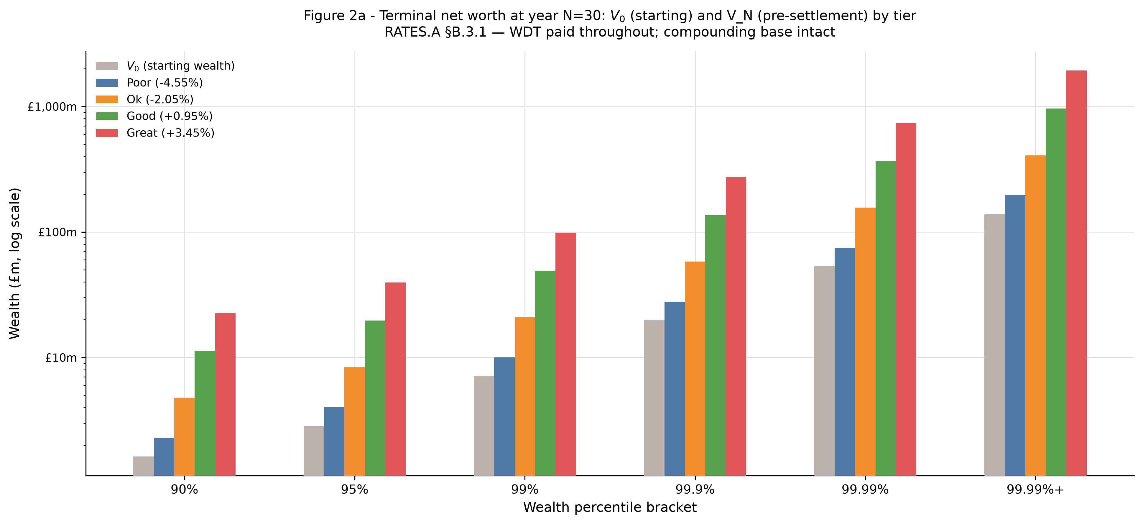
The WDT does not progressively exhaust the wealth it taxes. A taxpayer at the 95th percentile starting with £2.858m reaches £39.54m after 30 years in the Great tier and £19.72m in the Good tier, having paid WDT throughout; at the 99th percentile, starting wealth of £7.135m becomes £98.71m and £49.21m respectively. In every cell the terminal figure is a substantial multiple of starting wealth: the mechanism taxes the annual increment at progressive marginal rates, not the stock, and the symmetric refund mechanism returns a proportional share of loss-year declines. The WDT reaches wealth as it grows; the compounding base remains intact throughout.
The matrices below present both metrics at the reference calibration: Balanced parameters (\(\tau_0\) = 15%, \(\tau_m\) = 70%, \(k\) = 0.001 per £m, \(W_{min}\) = £2m), computed at the canonical 30-year burden horizon (N=30). The 2000 scenario drives the historical return sequence used; the burden figures are calibrated to N=30 across all scenarios to provide a consistent long-run comparison. A different return series or finer historical granularity would produce different figures. The full sensitivity results are in (RATES §7.2) and (RATES.A §B.4).
Annual wealth burden: tax paid as % of existing net worth — N=30
| Growth tier / Wealth percentile | 50% | 60% | 70% | 80% | 90% | 95% | 99% | 99.9% | 99.99% | 99.99%+ |
|---|---|---|---|---|---|---|---|---|---|---|
| −4.55% (Poor) | 0.00% | 0.00% | 0.00% | 0.00% | 0.12% | 0.17% | 0.17% | 0.17% | 0.18% | 0.20% |
| −2.05% (Ok) | 0.00% | 0.00% | 0.13% | 0.21% | 0.31% | 0.32% | 0.32% | 0.33% | 0.34% | 0.39% |
| +0.95% (Good) | 0.18% | 0.27% | 0.31% | 0.36% | 0.40% | 0.41% | 0.42% | 0.43% | 0.47% | 0.59% |
| +3.45% (Great) | 0.33% | 0.37% | 0.40% | 0.42% | 0.44% | 0.45% | 0.46% | 0.49% | 0.57% | 0.79% |
| Aggregation | Value | Basis |
|---|---|---|
| Population-weighted average | 0.24% | Each taxpayer counted once; lower-wealth brackets dominate numerically |
| Revenue-weighted average | 0.35% | Tax as fraction of aggregate terminal wealth; higher-wealth brackets dominate |
Directly comparable to stock-based wealth tax rates. Most proposed wealth taxes are levied at 1–2% of net worth annually; the WDT’s revenue-weighted burden of 0.35% reflects the delta base — only annual growth is taxed, not accumulated stock.
Effective rate on gains: tax paid as % of lifetime wealth increase — N=30
| Growth tier / Wealth percentile | 50% | 60% | 70% | 80% | 90% | 95% | 99% | 99.9% | 99.99% | 99.99%+ |
|---|---|---|---|---|---|---|---|---|---|---|
| −4.55% (Poor) | 0.0% | 0.0% | 0.0% | 0.0% | 10.9% | 15.6% | 15.7% | 15.9% | 16.5% | 18.2% |
| −2.05% (Ok) | 0.0% | 0.0% | 5.7% | 9.7% | 14.7% | 15.0% | 15.2% | 15.5% | 16.3% | 18.6% |
| +0.95% (Good) | 6.3% | 9.7% | 11.2% | 13.1% | 14.7% | 15.1% | 15.3% | 15.9% | 17.5% | 21.9% |
| +3.45% (Great) | 11.0% | 12.3% | 13.3% | 14.2% | 14.9% | 15.2% | 15.6% | 16.6% | 19.5% | 27.2% |
| Aggregation | Value | Basis |
|---|---|---|
| Population-weighted average | 9.1% | Each taxpayer counted once; cells with net lifetime loss excluded |
| Gain-weighted average | 13.0% | Tax as fraction of aggregate lifetime wealth created; higher-wealth brackets dominate |
Directly comparable to CGT or income tax rates on gains. The gain-weighted figure of 13.0% is the closer analogue to a statutory rate applied to aggregate gains — it represents total WDT collected as a fraction of total lifetime wealth increase across the modelled population. Cells showing 0.0% received net refunds over the horizon; the WDT issued a net payment to these taxpayers, not a charge.
Growth tier differentials are persistent adjustments relative to the UK historical average equity return of 10.45% per annum; implied returns are 5.90%, 8.40%, 11.40%, and 13.90% respectively. See (RATES §5.2). In years of negative return, the symmetric refund mechanism produces a net payment from the state to the taxpayer, reducing the lifetime average.
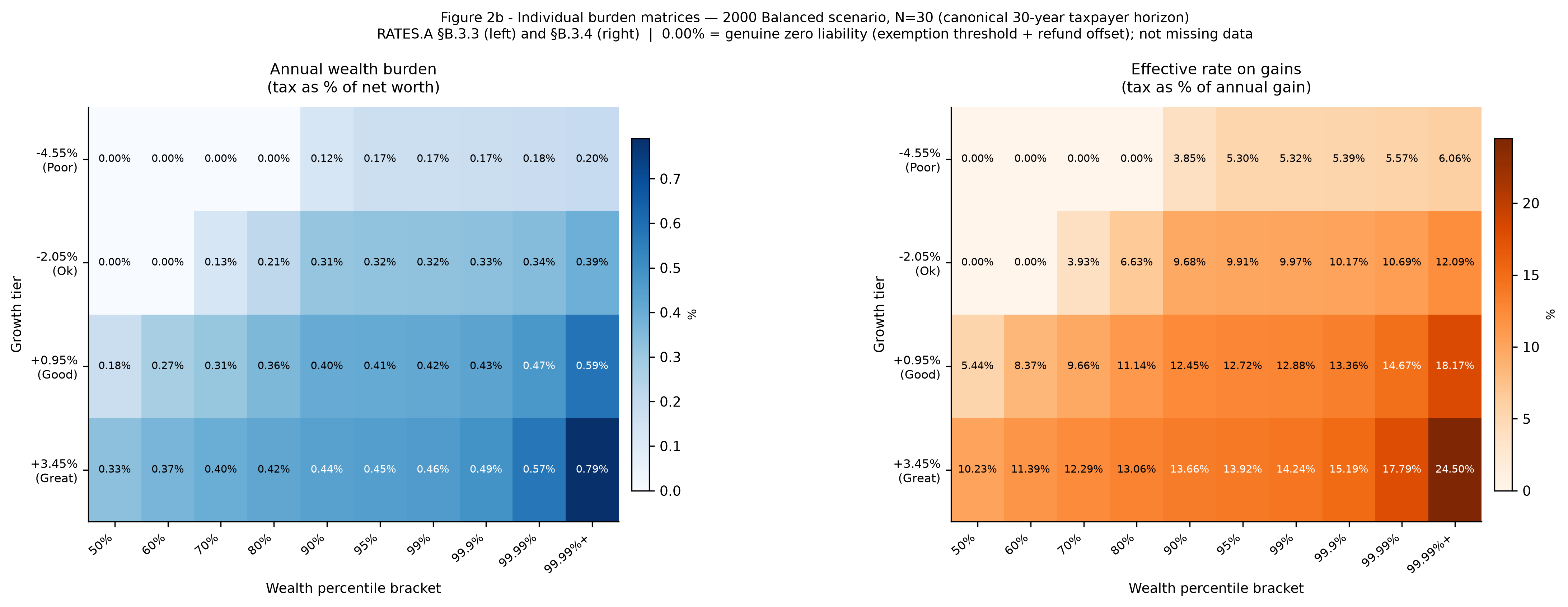
The heatmap makes the dominant gradient visible in a way the tables do not: burden rises far more steeply across tiers (moving down the grid) than across wealth brackets (moving right). The logistic rate function’s ceiling prevents the bracket dimension from diverging sharply at the top end, while persistent return differentials compound throughout the 30-year horizon to drive the tier dimension. The 0.00% cluster in the lower-left corner of each panel is the symmetric refund mechanism working as intended: below-average growth tiers at lower wealth brackets generate modest gain-year liabilities offset by loss-year refunds, leaving a zero or near-zero lifetime net. The maximum values — 0.79% wealth burden and 27.2% effective rate on gains — are isolated in the single top-right corner cell, requiring simultaneous membership of the highest wealth bracket and highest growth tier over the full horizon.
The aggregation rows supply the comparisons that make these figures policy-legible. On the wealth burden dimension, the population-weighted average across all modelled taxpayers is 0.24% of net worth per year; the revenue-weighted average (tax as a share of aggregate terminal wealth, where larger holdings count more) is 0.35%. Most proposed stock-based wealth taxes are levied at 1–2% of net worth annually, applied to the full accumulated stock regardless of whether it grew in that year. The WDT’s revenue-weighted burden of 0.35% sits well below that range — not because the mechanism is less ambitious, but because taxing the annual delta rather than the stock is a structurally different and structurally lighter charge on the same population. A taxpayer whose wealth does not grow in a given year pays nothing and receives a refund if it falls.
On the gains dimension, the population-weighted average effective rate on lifetime gains is 9.1%; the gain-weighted average — total WDT collected as a fraction of total lifetime wealth increase across the modelled population — is 13.0%. The gain-weighted figure is the correct analogue to a statutory CGT or income tax rate applied to aggregate gains, since it weights each taxpayer’s rate by the size of their gain rather than counting each taxpayer equally. UK CGT applies at 18% or 24% on realisation, but only to the fraction of appreciation crystallised in a taxable disposal. The WDT’s gain-weighted effective rate of 13.0% applies to every pound of annual appreciation whether or not it is realised — it reaches unrealised gains that CGT never touches. The relevant comparison is therefore not 13.0% versus 24%, but 13.0% on a substantially larger base versus a rate that is routinely reduced through deferral, relief structures, and the legal avoidance vehicles available to the WDT population, versus a WDT that admits no equivalent reduction.
The zero entries in the Poor and Ok tiers at lower wealth brackets reflect the interaction of actual historical return volatility with the symmetric refund mechanism. Using the actual UK equity return sequence rather than a smooth compound growth path, taxpayers in below-average growth tiers at lower wealth levels generate modest gain-year liabilities that are partially or fully offset by loss-year refunds. The result is a zero or near-zero lifetime average — the mechanism functioning as designed.
The maximum annual wealth burden across the entire modelled population at 2000 Balanced parameters is 0.79% of net worth per year, a ceiling requiring simultaneous membership of the top 0.01% wealth bracket and the highest persistent-outperformance growth tier across the canonical 30-year burden horizon. For most taxpayers the annual burden is a fraction of a percent of existing wealth.
The tax base is the annual increment, not the stock. A taxpayer whose wealth grows at 12% per annum and whose marginal rate is 35% faces a liability of 35% × 12% \(\approx\) 4.2% of annual growth, or approximately 0.5% of net worth. That arithmetic is what produces the 0.35% revenue-weighted burden average despite rates that rise to 70% at the ceiling: the ceiling applies to the delta, not the stock, so even aggressive progressive rates translate into sub-percent annual burdens at population scale.
The effective rate on gains rises with both wealth and growth experience. A taxpayer at the 50th percentile in the Good tier pays a 6.3% effective rate on lifetime gains; one at the top 0.01%+ bracket in the Great tier pays 27.2%, because the rate function applies progressively to both a larger delta and a faster-compounding base. The maximum effective rate on gains of 27.2%, at the very top of both distributions, is a lifetime average over 30 years that includes both gain years and loss years with refunds; it is not a single-year figure. The WDT taxes persistent outperformance compounding at scale, which is the foundational claim in (MF §4).
All figures are pre-behavioural. Revenue is heavily concentrated at the upper tail (roughly the 99.9th percentile and above) — the population most capable of responding. The behavioural-modelling paper (BEHAV) addresses this; the figures here are the pre-response baseline.
3. The Revenue Claim
The central revenue claim of this paper is directional and order-of-magnitude rather than precise. At the 2000 reference calibration (Balanced parameters: \(\tau_0\) = 15%, \(\tau_m\) = 70%, \(k\) = 0.001 per £m, \(W_{min}\) = £2m) applied to the UK equity return data, the WDT demonstrably delivers meaningful post-fill labour-relief surplus as a fraction of UK government expenditure. The relevant window is not the capitalisation phase (during which reserves are still being built and existing taxes remain in place) but the years after LRR fill, when the mechanism is self-sufficient and surplus Step-5 revenue is available for fiscal replacement.
Two post-fill coverage metrics bracket the plausible range. The SSM post-fill coverage applies the correlated-shock assumption (every taxpayer experiencing the same return simultaneously) and provides the floor; the TCM post-fill coverage applies heterogeneous persistent tier differentials and provides the ceiling. At the 2000 reference scenario and a 10-year post-fill window, the SSM floor is 6.4% and the TCM ceiling is 14.6%. These are the most conservative figures in the sweep: 2000 produces the lowest 10-year TCM post-fill coverage of all 73 start years and is chosen as the reference precisely for that reason. Neither figure is more correct than the other; they stress different aspects of the same mechanism and together bracket the plausible range. The full specification is in (RATES.A §A.6).
The historical starting-year sensitivity analysis in (RATES §7.2) confirms that meaningful post-fill coverage holds across all historical starting conditions. Across all 73 start years in the 1947–2019 UK equity return data, the 10-year TCM post-fill coverage ranges from 14.6% (2000 start) to 321.4% (1970 start), with a median of 125.5%. Several start years from the 1960s and early 1970s produce 20-year TCM coverage exceeding 300%. The mechanism is capable of replacing appreciable fractions of government expenditure within a decade of LRR fill under all historical starting conditions, and exceeds 100% of annual expenditure within 20 years at the median start. The 2000 reference produces the lowest 10-year figures; the magnitude claim is robust precisely because even the hardest case remains in the material tens of percent. For specific context, UK annual expenditure at LRR breakeven (year 19) is £2,560b (RATES.A §B.2), compared to a 2022–23 base of £1,157b (JUR §2.2).
The 2000 reference is deliberately the worst case, not the expected case. The median start year produces a 10-year TCM post-fill coverage of 125.5% — meaning the WDT would, under most historical return environments, have been capable of replacing government expenditure in full from surplus WDT revenue alone within a decade of self-sufficiency. Choosing the minimum as the reference is an analytical decision: every claim in this paper rests on the floor of the historical distribution. The centre of that distribution is not suppressed; it is the benchmark against which the floor should be read.
3.1 Direction of Conservatism
All modelling assumptions are chosen to understate rather than overstate revenue, with one exception. The Pareto distribution is calibrated from WAS anchor points that systematically undersample individuals above £3m, producing a lighter tail than the true distribution. This bias operates in two directions simultaneously. On the revenue side, a lighter modelled tail understates the tax base. On the liability side, it also understates refund exposure in crash years, since extreme-wealth taxpayers claiming symmetric refunds on large losses are underrepresented by the same degree. The SSM’s correlated-shock stress test should be read with this in mind: refund pressure in a 2008-analogue year is likely somewhat larger than the model assumes, for the same reason revenue in normal years is likely somewhat larger.
The taxable population is treated as a fixed cohort with no new entrants, despite new entrants generating large first-year deltas as their full stock above \(W_{min}\) enters the base. The four growth tiers assign 40% of taxpayers to below-average differentials despite Fagereng et al. (2020) finding a positive wealth-return correlation; the WDT population, concentrated in the upper deciles, likely contains more Good and Great tier investors than the model assumes. The assessment window premium, corporate levy, and ultra-high-net-worth tail are all excluded from the reference estimate and are addressed in (RATES §8).
One assumption runs against the conservative direction, and it is the most consequential: behavioural responses are not modelled. Migration, restructuring, and avoidance will reduce actual revenue by an amount unknown at this stage; this is the primary source of overstatement in the reference figures and is assigned to BEHAV. However, it does not follow that the net direction of bias is unambiguously upward. A taxpayer who migrates removes themselves from both the tax base and the refund pool; a restructured asset that escapes WDT also forfeits refund entitlement in loss years. The conservative assumptions on the revenue side and the overstating assumption on the behavioural side partially offset each other at the margin. The net bias direction is uncertain rather than clearly upward — which makes Phase One evidence-gathering a necessary analytical step rather than merely a precautionary one.
One input carries significant denominator weight without being sensitivity-tested. The expenditure growth rate of 4.51% per annum, derived from historical UK Total Managed Expenditure 1999–00 to 2019–20 (HM Treasury, 2024, Table 10; see (JUR §2.11) for derivation), determines how large the fiscal obligation is at each point in the capitalisation window. If real expenditure growth trends higher than this (plausible under sustained demographic pressure, defence spending increases, or health system cost growth) post-fill coverage fractions fall. The direction of this risk is clear; its magnitude is not. The historical starting-year sensitivity analysis in (RATES §7.2), while not a direct test of the expenditure growth rate, confirms that the tens-of-percent magnitude claim holds across a wide range of starting conditions.
4. The Rate Function
The WDT applies a logistic marginal rate function to the annual wealth delta, rising smoothly from a minimum floor to an asymptotic ceiling. Rate structure is a political question settled through the Governing Council; the function is specified by four parameters: \(\tau_0\) (floor rate), \(\tau_m\) (asymptotic ceiling), \(k\) (steepness, in per £m), and \(W_{min}\) (entry point in millions of pounds).
\[ \tau(W)=\frac{\tau_m}{1+\left(\frac{1-\tau_0}{\tau_0}\right)e^{-k(W-W_{\min})}} \]
Full symmetry of the loss-refund mechanism is a settled design position, not a parameter. Partial symmetry (refunding losses at a rate below the applicable marginal gain rate) fails on two distinct grounds. Mechanically, it breaks the Domar & Musgrave (1944) risk-sharing logic: the government functions as a proportional partner in the taxpayer’s risk only when it absorbs losses at the same rate it captures gains. On foundational grounds (MF §6); (MF §7), the symmetric refund is the operational expression of the state accepting downside exposure alongside the taxpayer; partial symmetry abandons that commitment rather than calibrating it. Formal numerical modeling is undertaken in (WFR).
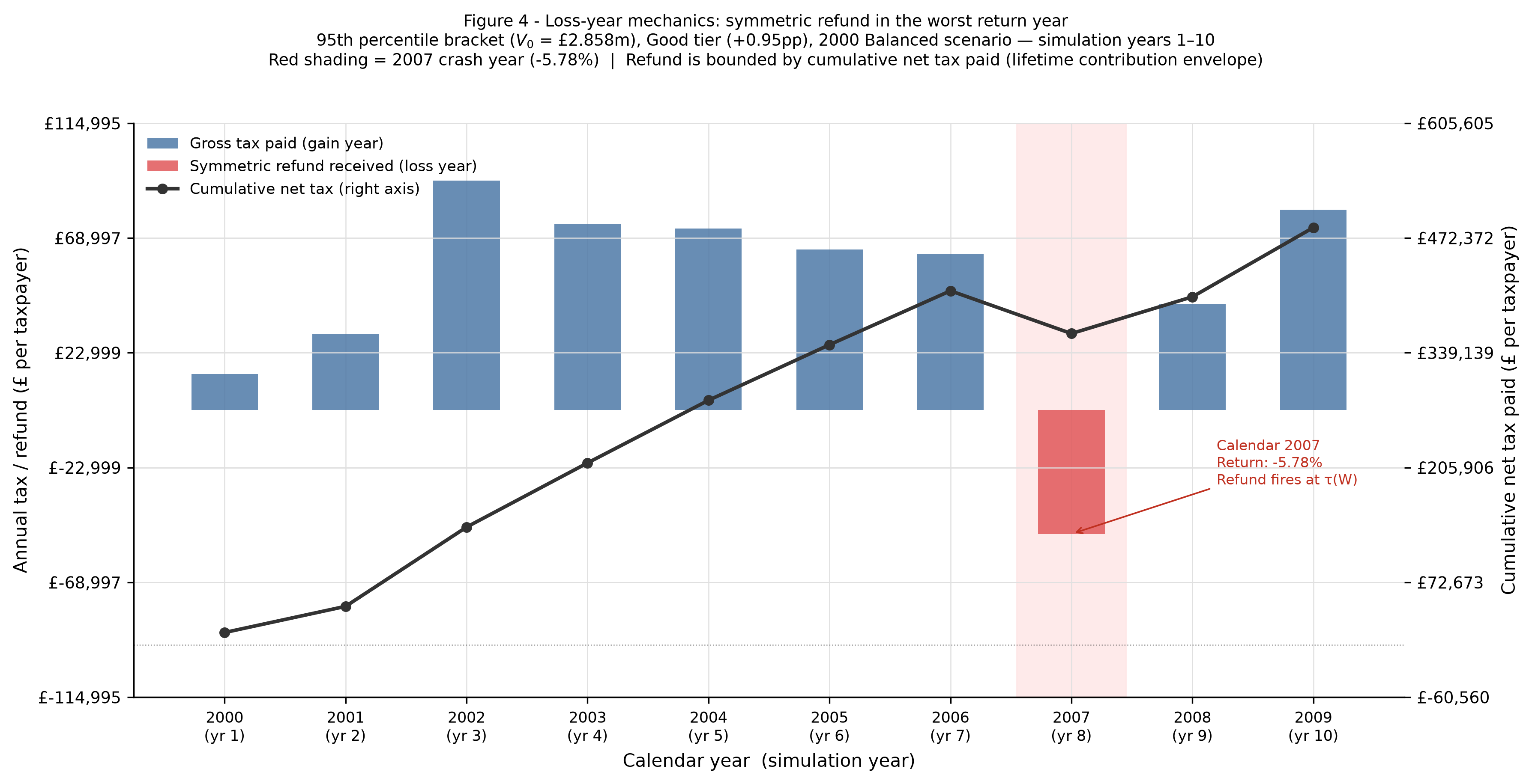
Figure 8 shows what full symmetry delivers at the individual level across the first ten years of the 2000 scenario, for a representative taxpayer at the 95th percentile bracket in the Good tier. In gain years the mechanism collects gross tax at the applicable marginal rate; in simulation year 8 (calendar 2007, the crash year in this rotated series) the refund fires at the same rate \(\tau\)(W) that would have applied to an equivalent gain. The cumulative net tax line confirms the lifetime contribution envelope is respected throughout: the refund in year 8 reduces cumulative net tax paid but does not bring it below zero, because taxes paid in years 1–7 are sufficient to cover the refund. The envelope constraint is binding from above, not below: the mechanism cannot pay out more in refunds than has been paid in taxes over the lifetime horizon. This is the Domar-Musgrave partnership made concrete — the state participates in the downside of the crash, proportionally, at the same rate it would have captured the upside.
The lifetime contribution envelope performs a structural role beyond protecting the taxpayer from net extraction. Because cumulative refunds are capped by cumulative taxes paid, a taxpayer with a short history of prior gains can only claim a small refund in a crash year regardless of the size of the loss. This limits unplanned SRR drawdown precisely when the SRR is most stressed: in early-year crashes, when the population’s tax history is thin, refund exposure is automatically bounded by that history. The mechanism is self-limiting without any active Governing Council intervention — which is useful because interventions are hardest to execute during a simultaneous market shock.
The envelope also closes a specific fraud vector. Without it, a participant could manufacture paper losses, claim the symmetric refund, then exit the country before paying taxes sufficient to cover that refund. With the envelope in place, such an exit produces at worst a zero net position: the refund cannot exceed taxes already collected. The cost of attempting this attack is the full prior tax history, which scales with how long the participant has been in the system.
The Governing Council retains discretion to modify the envelope at the margin. Two variants warrant noting as available options, neither of which is a current design position. First, the cap could be lifted entirely — allowing refunds to exceed lifetime taxes paid. This would deepen the SRR’s exposure in crash years but could serve as a political concession during the bootstrapping phase, signalling a stronger state commitment to the downside partnership. It would require separate legal architecture to close the fraud surface: exit charge clawback, residency bond requirements, or a minimum holding period before full refund eligibility. Second, a negative floor restriction could permit moderate net refund positions up to a defined ceiling (for example, allowing refunds to exceed taxes by up to a fixed percentage of terminal wealth), with proportional legal protections against manufactured losses. Either variant is structurally compatible with the WDT mechanism and could be offered as a targeted Phase One concession for the taxpayer population whose early buy-in matters most politically.
The assessment window premium is excluded from the reference revenue model entirely. The mechanism functions without it, making exact rates a Phase One calibration question. The deferral charge is anchored to sovereign borrowing cost; the flexibility levy is calibrated against Phase One election data. Both are set by the Governing Council under its Tier 1 process (GOV §6) once that evidence exists.
The corporate rate-floor question (OQ #30) is not settled by this paper. The full derivation is in CORP.A §B.1–B.2, which disaggregates the question into two distinct optimisation problems: \(\tau_{prov}\) (an administrative cash-flow parameter) and \(\tau_h\) (a final charge on permanently unattributable ownership). Under that framework, \(\tau_m\) is the ceiling of the plausible range for \(\tau_h\) rather than a predetermined anchor. The revenue model in (RATES §8.1) retains \(\tau_c\) = \(\tau_m\) = 70% as the working ceiling assumption for estimation purposes.
5. Modelling Wealth and Its Growth
5.1 The Wealth Distribution
The model combines WAS-observed decile data for the bottom 99% of the UK adult population with a Pareto extrapolation above the top-1% threshold of £3.6m. The calibration uses two WAS anchor points: the top-1% threshold (£3.6m, N = 692,000) and the top-0.1% threshold (£10m, N = 69,200). The tail exponent is estimated at \(\alpha\) = 2.2538; the model uses \(\alpha\) = 2.25. \(W_{min}\) is a rate design parameter determining where the rate function produces material liability, not a population boundary.
| Bracket | N | Mean wealth | Agg. wealth (£b) |
|---|---|---|---|
| 0–10th pct | 6,920,000 | £3,474 | £24.0 |
| 10–20th pct | 6,920,000 | £23,080 | £159.7 |
| 20–30th pct | 6,920,000 | £68,512 | £474.1 |
| 30–40th pct | 6,920,000 | £147,026 | £1,017.4 |
| 40–50th pct | 6,920,000 | £261,108 | £1,806.9 |
| 50–60th pct | 6,920,000 | £401,789 | £2,780.4 |
| 60–70th pct | 6,920,000 | £569,543 | £3,941.2 |
| 70–80th pct | 6,920,000 | £782,141 | £5,412.4 |
| 80–90th pct | 6,920,000 | £1,108,535 | £7,671.1 |
| 90–95th pct | 3,460,000 | £1,629,190 | £5,637.0 |
| 95–99th pct | 2,768,000 | £2,858,347 | £7,911.9 |
| Top 1%–0.1% | 622,800 | £7,135,016 | £4,443.7 |
| Top 0.1%–0.01% | 62,280 | £19,853,605 | £1,236.5 |
| Top 0.01%–0.001% | 6,228 | £53,384,707 | £332.5 |
| Top 0.001%+ | 692 | £139,607,368 | £96.6 |
| Total (WAS, below top 1%) | 68,508,000 | £36,836.1 | |
| Total (Pareto, top 1%+) | 692,000 | £6,109.3 | |
| Grand total | 69,200,000 | £42,945.4 |
Source: ONS WAS 2018–20 (below top 1%); Pareto extrapolation (top 1% and above). Above the top-1% threshold, all figures are Pareto-implied.
The Pareto-implied population at the top-10% threshold falls within 3.5% of the WAS-observed figure. The WAS undersamples above £3m, so the modelled tail is almost certainly lighter than the true distribution. The practical upper bound of approximately £140m at the top 0.001% bracket lies far below the actual holdings of the UK’s wealthiest individuals; that gap is addressed in (RATES §8.2). The aggregate revenue result is effectively insensitive to the Pareto tail exponent \(\alpha\) across the full plausible range (2.00 to 2.40), because the tax base is the annual delta rather than the stock: small changes in tail shape shift the wealth distribution modestly without materially changing the flow of annual increments.
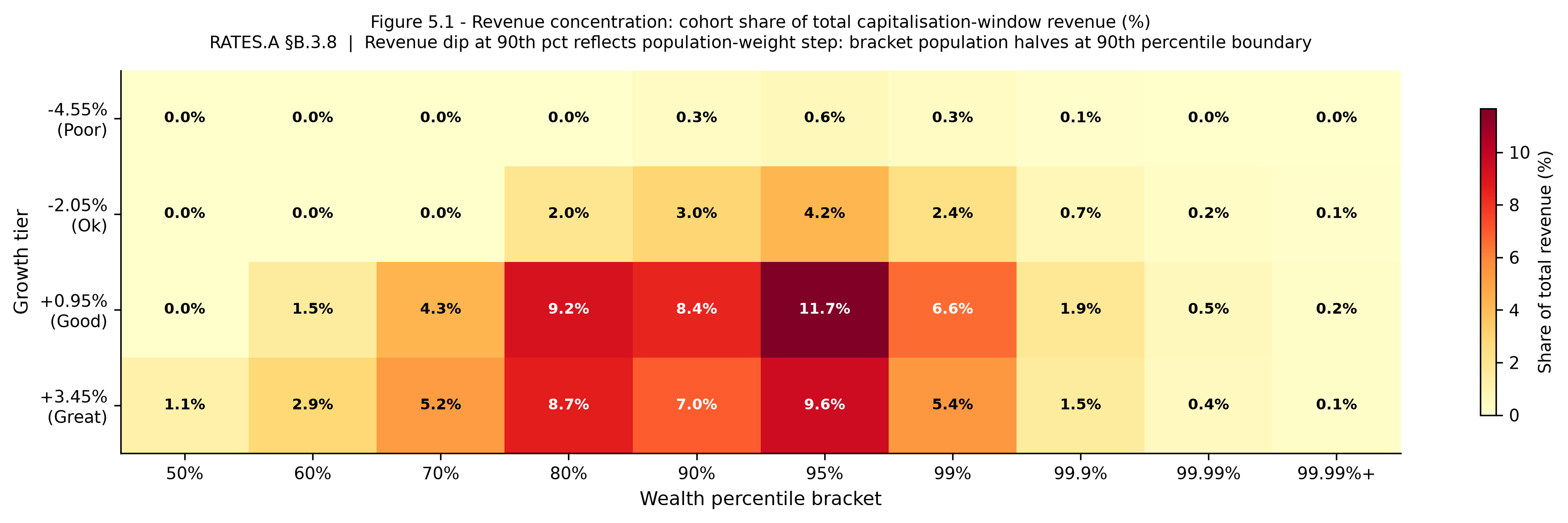
Where aggregate revenue concentrates does not follow straightforwardly from the wealth distribution alone. The Good tier (40% of taxpayers) fields 2,768,000 participants across the 50th to 80th percentile brackets; the Great tier (20%) fields only 138 in the top 0.001% bracket (RATES.A §B.3). Volume and growth rate combine rather than substitute: the mid-to-upper brackets contribute the bulk of aggregate revenue not because individual liabilities are highest there but because population counts remain substantial at brackets where the rate function produces material liability. The revenue concentration results in (RATES §7.1) follow from this structure.
5.2 The Growth Model
The tax base is the annual delta rather than the stock, so revenue depends on how wealth grows, not just how much is held. The historical mean return is derived from 73 years of UK equity capital total return data (1947–2019): 10.45% per annum (Jordà et al., 2019).
Fagereng et al. (2020) document, from 20 years of Norwegian administrative records, that individuals earn persistently different returns on net worth, with a standard deviation of 8% and substantial persistence (LR.B §5). Returns are positively correlated with wealth: moving from the 10th to the 90th percentile of the wealth distribution increases financial asset returns by 3 percentage points, even within asset classes.
The model adopts four persistent growth tiers, expressed as differentials relative to the historical mean of 10.45%:
| Tier | Population share | Differential vs mean | Implied return |
|---|---|---|---|
| Poor | 10% | −4.55pp | 5.90% |
| Ok | 30% | −2.05pp | 8.40% |
| Good | 40% | +0.95pp | 11.40% |
| Great | 20% | +3.45pp | 13.90% |
The population-weighted average recovers 10.45%. The 800 basis-point spread is consistent with Fagereng et al.’s reported dispersion. The weights are conservative: assigning 40% of taxpayers to below-average tiers overstates the underperforming share of a population drawn from the upper deciles, given Fagereng et al.’s finding of a positive correlation between wealth and returns.
In the TCM, each taxpayer’s wealth in period t grows at the actual historical return for that period (taken from the UK equity return series rotated so that the active scenario’s start year sits at index zero) plus their tier’s persistent differential. Taxpayer cohorts therefore experience the same actual year-by-year return volatility as the SSM rather than a smooth compound path. The common return-sequence basis is what allows the SSM and TCM to be read together: both models operate on the same historical data, differing only in whether returns are applied uniformly across the population (SSM) or heterogeneously by tier (TCM). The marginal cohort architecture that enables this is described in full in (RATES.A §A.2).
6. The Two Models and How They Connect
The SWF Solvency Model (SSM) is a transition-planning instrument tracking year-by-year how the UK government moves from its current tax base to a WDT-funded settlement. The SSM applies actual historical UK equity returns uniformly to the entire taxable population in each year (the worst-case assumption for simultaneous refund pressure) and deliberately excludes heterogeneous growth tiers. The objective is to stress the system against correlated shocks, not to estimate expected revenue.
The Taxpayer Cohort Model (TCM) is calibrated to the LRR breakeven year as its modelling horizon. For each of ten wealth percentile brackets and four growth tiers, it computes cumulative tax paid and refunds received by a representative taxpayer starting at the mean bracket wealth and following the relevant growth path over N periods. In each period, wealth grows at the actual historical return for that period plus the tier’s persistent differential. The annual delta is the change in wealth from the prior period’s declared basis. The rate function is applied to positive deltas to compute gross tax; in loss years the symmetric refund mechanism produces a refund at the same marginal rate, subject to the lifetime contribution envelope. Results are population-weighted across all cells and divided by N to produce the annual average revenue figure.
The two models share all rate parameters, wealth distribution calibration, and growth assumptions, differing only in one dimension: the SSM applies uniform historical returns; the TCM applies heterogeneous persistent tier differentials to the same rotated return series. The SSM establishes when the mechanism becomes self-sufficient; the TCM evaluates what it delivers during the capitalisation window and at maturity. The LRR breakeven year (the first year the LRR balance reaches the 3× expenditure capitalisation floor) is the input connecting them.
6.1 Sizing the SRR
The SRR’s target balance is not derived from the theoretical refund ceiling alone. That ceiling (the maximum liability if all taxpayers simultaneously claimed maximum refunds with no offsetting tax income) is astronomically large and would take decades to reach in any scenario. The operational sizing target is the SRR capitalisation ratio: the SRR target balance as a multiple of net annual WDT income under normal conditions. The recommended Governing Council floor is 3×. The 3× figure is chosen to be achievable within a single political cycle from launch, providing an early credibility milestone without requiring an implausibly long capitalisation phase. It is a Governing Council parameter under the Tier 1 process (GOV §6), not a fixed design constant.
The SRR sizing is expressed in units of observed net annual WDT revenue, not in units of any predicted declaration ratio. The TCM computes revenue by applying the rate function to population-weighted deltas across all brackets and growth tiers; the 3× capitalisation target is then a multiple of that revenue figure. The declaration ratio \(\alpha\) does not appear as an explicit input. The SRR’s response to population-level declaration behaviour is therefore automatic and endogenous: if the population systematically overstates (\(\alpha\) > 1), declared deltas are larger than true deltas, gross revenue is correspondingly higher, and the 3× target fills at a faster pace than the \(\alpha\) = 1 baseline model implies. If the population systematically understates (\(\alpha\) < 1), the reverse holds and fill is slower. The Governing Council does not need to estimate the population \(\alpha\) in advance or build an explicit correction into the SRR target. The calibration self-adjusts to whatever declaration behaviour the system produces, and Phase One data on declared values relative to realisation prices (PHASE1 §5.4) will provide the first empirical basis for assessing whether the revenue stream reflects systematic deviation in either direction. The ENV §2 observation that a mild-overstatement equilibrium near \(\alpha\) \(\approx\) 1.1 would call for a modestly upward SRR calibration should be read as a directional note for the Governing Council’s first post-Phase-One review, not a pre-launch sizing requirement.
The robustness claim the model makes about the SRR concerns what happens when it does breach. It breaches in 41 of 73 start years in the historical sweep; in every case the LRR balance at the moment of first breach is sufficient to cover the SRR deficit in full. The full breach coverage results are in (RATES.A §B.4) and (RATES.A §B.5). Across all 73 start years the SRR fill year is invariant at 3, a robustness result addressed further in (RATES.A §B.5).
6.2 Sizing the LRR
The LRR’s failure mode is structurally different from the SRR’s and requires a different sizing logic. The SRR faces a contingent liability (refunds) whose magnitude is bounded and calculable. The LRR faces a fixed and growing obligation (annual government expenditure) that does not respond to poor returns. The SRR’s problem is a spike in claims; the LRR’s problem is a revenue drought against an obligation that does not shrink.
The appropriate measure is a buffer against the cumulative revenue shortfall in a sustained bad-return sequence: how many years of expenditure could the LRR cover if WDT revenues fell to zero. A floor expressed in years of expenditure is legible, structurally motivated, and consistent with how sovereign reserve funds are conventionally sized against contingent fiscal obligations.
The recommended LRR floor is 3 years of government expenditure at the prevailing annual rate. At the 2000 Balanced scenario breakeven (year 19), annual expenditure has reached £2,560b; the 3× floor at that point is £7,680b, against which the LRR carries a surplus of £104b. Like the SRR capitalisation ratio, this is a Governing Council parameter. The Governing Council may revise it upward through the Tier 1 process as Phase One behavioural data accumulates.
UK government expenditure growth is modelled at 4.51% per annum, derived from the historical UK Total Managed Expenditure series 1999–00 to 2019–20 (HM Treasury, 2024, Table 10; see (JUR §2.11) for the corrected derivation). Its effect on the revenue claim is noted in (RATES §3.1): a higher expenditure growth rate raises the fiscal hurdle the mechanism must clear, making post-fill coverage fractions in the material tens of percent a stronger demonstration of viability.
6.3 The Two Internal Milestones and What They Gate
Because the SRR and LRR fill on different timescales, Phase One contains an internal inflection point rather than a single end date. The two milestones are conceptually and operationally distinct.
SRR fill occurs within 3 years at the 2000 reference scenario. It marks the moment the refund guarantee becomes credible: the state has pre-funded its symmetric loss commitment and the cooperative architecture’s claim — that the WDT is a partnership backed by reserves rather than an aspirational promise — is mechanically substantiated. Before SRR fill, the symmetric refund is a promise backed by future revenue; after it, the promise is backed by a ring-fenced reserve that has survived the historical stress test. Across all 73 start years in the historical sweep, the SRR fill year is invariant at 3; this near-invariance is addressed in (RATES §7.2).
LRR fill occurs at year 19 in the 2000 reference scenario, and at a median of 13 years across the full 73-start-year sweep. It marks the moment the LRR balance reaches the recommended capitalisation floor, at which point fiscal replacement is viable: the transition account can sustain annual government expenditure from WDT revenue alone without drawing on legacy taxes or exposing the LRR floor. This is the precondition for the labour tax relief dividend to be delivered at scale, the terminal goal identified in (WP §1.1) and (MF §6).
The post-fill coverage metrics measure what happens after this milestone rather than during the accumulation phase. Average annual lifetime TCM revenue at N=30 is £873.6b, substantially above the capitalisation-window average of £563.3b (see (RATES.A §B.3.9)); the 2000 scenario front-loads the dot-com bust and 2007 crash, depressing early-window revenue considerably relative to the long-run mean. This is precisely why the 10-year post-fill metric is the right frame for the revenue claim: it captures the mechanism’s performance in the first decade after self-sufficiency under the worst historical starting conditions available, without conflating that performance with the accumulation phase during which no fiscal replacement has yet occurred.
These milestones are economic events. Phase One and Phase Two are political terms describing the Governing Council’s chosen operating posture (the threshold level, rate structure, and population scope the system runs at) and are not defined by SRR or LRR fill. The Governing Council may adjust its operating posture before, after, or independently of either milestone. What the milestones supply is information: SRR fill tells the Governing Council that the refund guarantee is mechanically credible and that the case for modest tax relief has a reserve-backed foundation; LRR fill tells it that the transition account can sustain annual government expenditure from WDT revenue alone. Whether and when the Governing Council acts on either signal is a political decision the model does not determine.
Once the LRR target is met, continued accumulation at current rates is in tension with enumerated clause 6 (GOV §5.2), which commits net WDT revenue above pre-existing spending obligations to reducing taxes on labour and consumption, and with enumerated clause 4, which restricts the SWF’s capitalisation purpose to pre-funding the refund liability. A growing LRR beyond its stated floor is not pre-funding the refund liability; it is accumulating surplus that clause 6 requires to be directed elsewhere. Post-LRR-fill rate review is architecturally required by the governance design, not optional Governing Council housekeeping.
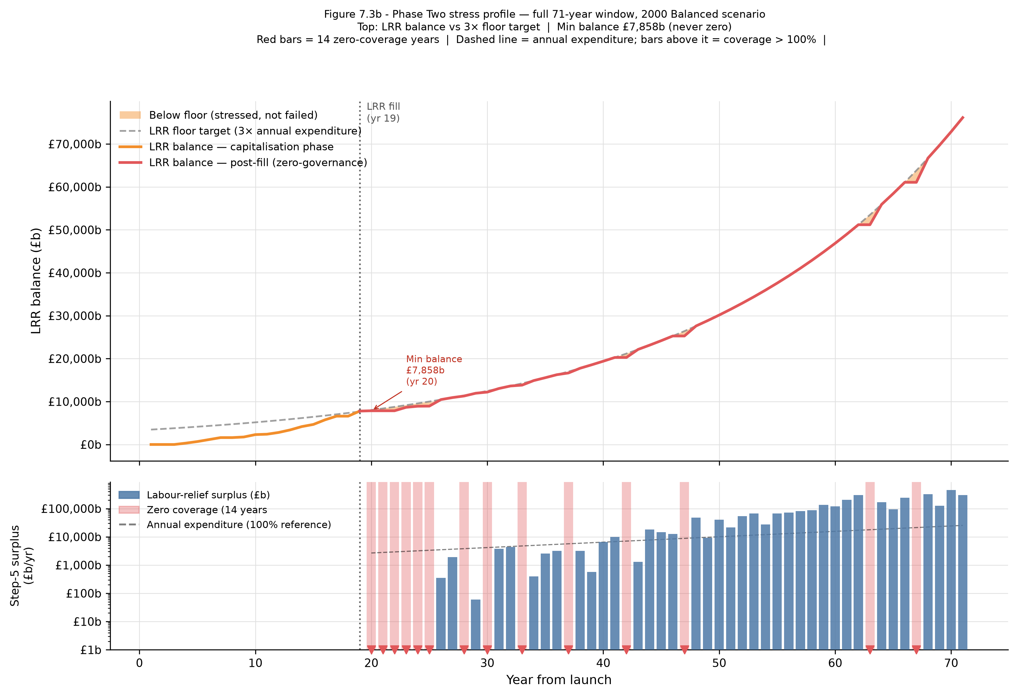
Figure 9 shows the full 71-year LRR profile for the 2000 scenario in two panels. The top panel tracks the LRR balance: the orange capitalisation phase accumulates toward the floor target, reaching it at year 19. Under the zero-governance assumption (red line), the LRR immediately dips below the 3× floor target as full annual expenditure is charged against the reserve — the amber shading marks years where the LRR is stressed but solvent, reaching a minimum of £7,858b at year 20 before WDT revenue on the compounding wealth base causes it to recover. The LRR never reaches zero. The bottom panel shows the Step-5 labour-relief surplus year by year: 14 years in which the surplus is fully consumed by Steps 1–4 (SRR maintenance and LRR floor restoration) appear as red bars, contributing zero to the post-fill coverage average; the remaining years show growing surplus available for fiscal replacement. The architectural obligation is binding from year 19 regardless of the zero-governance stress path: enumerated clause 6 requires surplus above the 3× floor to be directed to labour and consumption tax relief, not accumulated further. The mandatory rate review mechanism in (GOV §6) would in practice respond to the post-fill LRR dip well before it stressed the system materially, since the model makes no credit for governance response and the dip itself is shallow and self-correcting.
7. Revenue Results
7.1 Revenue Results and Coverage
At 2000 Balanced parameters (\(\tau_0\) = 15%, \(\tau_m\) = 70%, \(k\) = 0.001 per £m, \(W_{min}\) = £2m, N=19 cap. window / N=30 lifetime), the TCM produces total average annual revenue of approximately £873.6b over the canonical 30-year lifetime horizon, with a capitalisation window average (SRR fill to LRR fill, N=19) of £563.3b. The distribution across growth tiers is as follows.
| Growth tier | Lifetime avg N=30 (£b/yr) | Cap. window avg N=19 (£b/yr) |
|---|---|---|
| −4.55% (Poor) | £4.7b | £7.5b |
| −2.05% (Ok) | £77.4b | £70.6b |
| +0.95% (Good) | £374.7b | £248.9b |
| +3.45% (Great) | £416.8b | £236.1b |
| Total | £873.6b | £563.3b |
Revenue is concentrated in the upper brackets and higher growth tiers: the Good and Great tiers together account for approximately 91% of aggregate revenue. This makes the aggregate sensitive to the behavioural response of the population best positioned to respond: migration and avoidance among the most capable taxpayers. Those responses remain assigned to BEHAV; the figures here are the pre-response baseline.
Two post-fill coverage metrics express what the mechanism delivers in the years after LRR fill, when surplus Step-5 revenue is available for fiscal replacement. As established in (RATES §3), the SSM post-fill coverage provides the floor (correlated-shock assumption, maximising simultaneous refund pressure) and the TCM post-fill coverage provides the ceiling (persistent-heterogeneity assumption, where higher-tier taxpayers compound faster and generate higher average revenue). At the 2000 reference scenario and a 10-year post-fill window, the SSM floor is 6.4% and the TCM ceiling is 14.6%. The full specification and a known boundary-alignment limitation are in (RATES.A §A.6).
The 10-year window is the primary metric because it speaks directly to the near-term labour relief dividend: what fraction of government expenditure could the mechanism replace within a decade of becoming fiscally self-sufficient? At the 2000 reference — the hardest historical case — that fraction is between 6% and 15%. At the median start year, the 10-year TCM post-fill coverage is 125.5%, meaning the mechanism would have been capable of replacing government expenditure outright within a decade of LRR fill under most historical conditions. The parameters used here are one point in a large feasible space, not a recommendation.
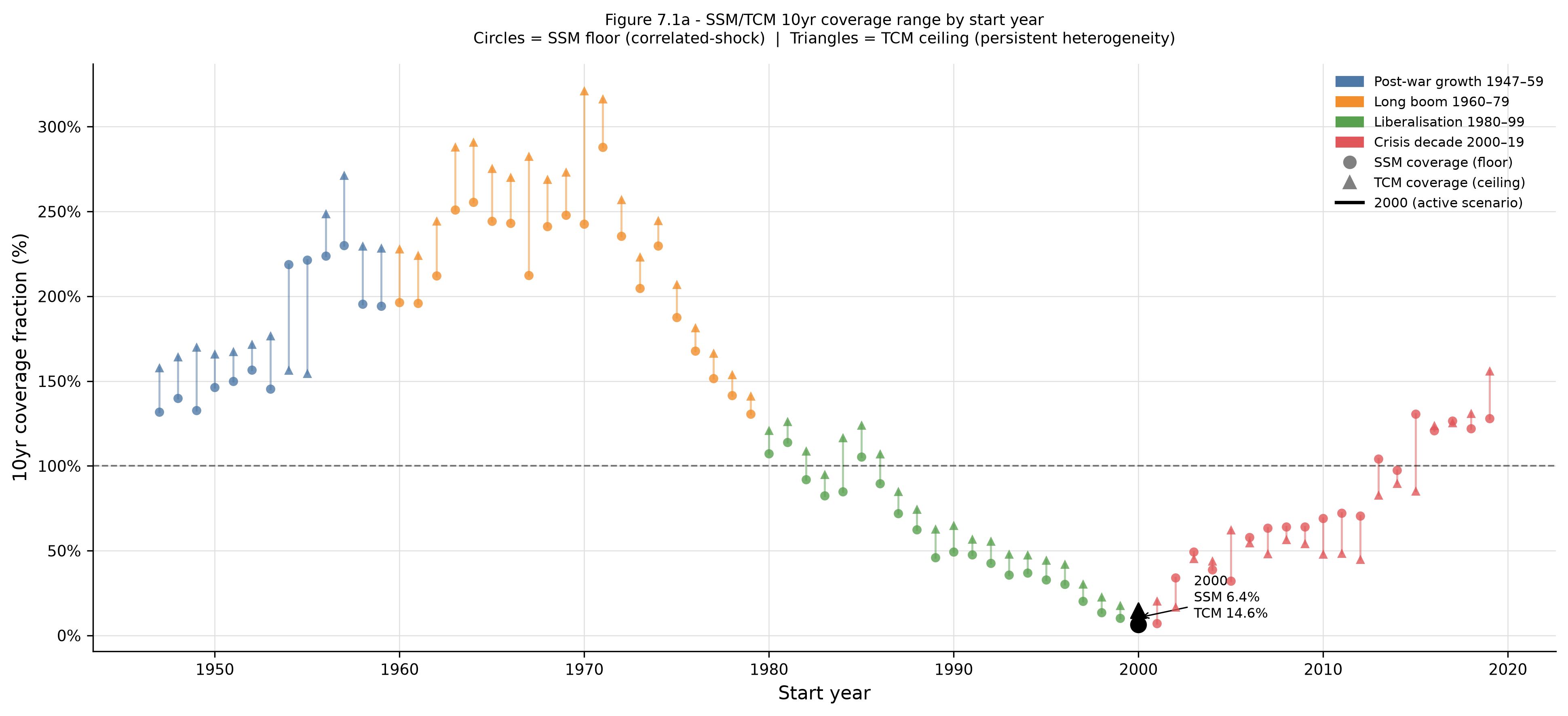
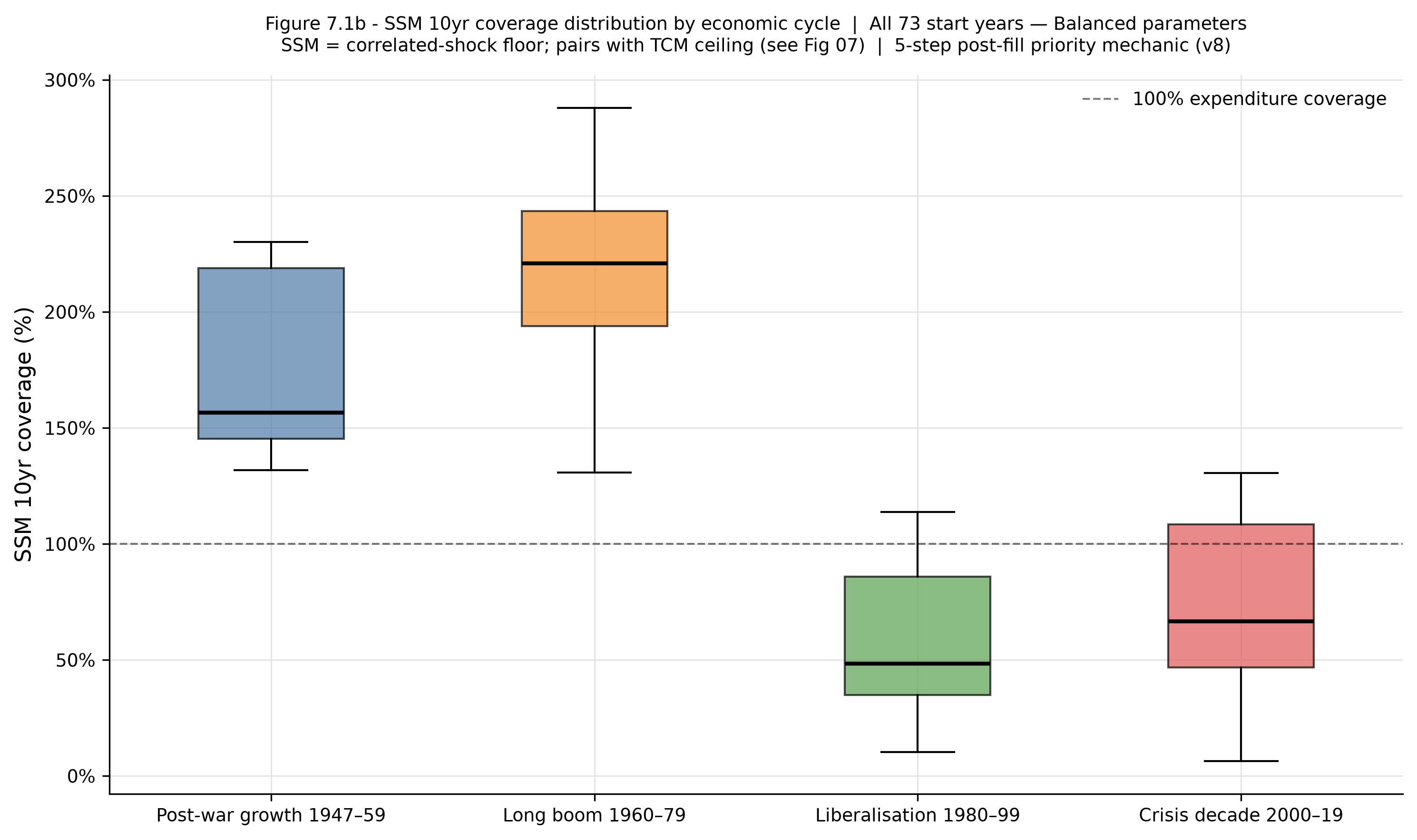
Figure 7.1 shows why the two-metric framework is necessary rather than convenient: the width of the SSM/TCM 10-year post-fill coverage band varies substantially by economic era. Bands are widest in the long-boom period (1960–79, orange), where high sustained mean returns amplify the effect of persistent tier differentials: when the mean is high, the Good and Great tiers compound faster in the post-fill years relative to the SSM’s uniform assumption, widening the gap between floor and ceiling. Bands narrow in the crisis decade (2000–19, red), where both floors and ceilings are lower and closer together, reflecting the depressed return environment and the concentration of bust years in the early post-fill period. The 2000 scenario (black, annotated) sits at the lower end of its era: SSM 6.4%, TCM 14.6% — the lowest pair in the full 73-start-year sweep. A single revenue figure for any start year would either misrepresent the floor or misrepresent the ceiling; the band is the honest characterisation of what the mechanism delivers under the two limiting distributional assumptions.
7.2 Historical Starting-Year Sensitivity
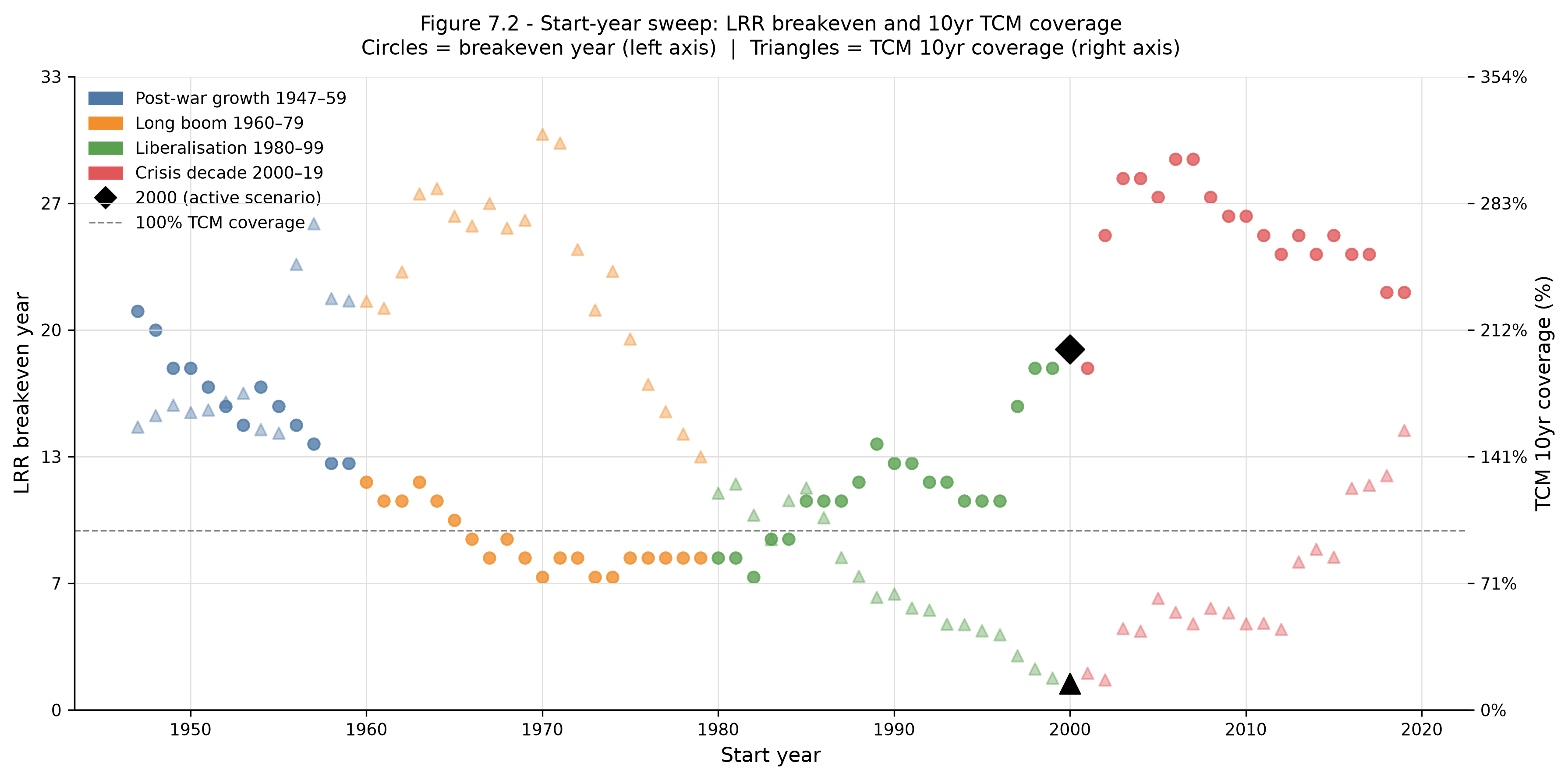
The 2000 reference scenario establishes what the mechanism delivers under the hardest illustrative case on the post-fill revenue dimension. To test whether the revenue and solvency results depend on that choice, the SSM was run at Balanced parameters from every viable start year in the 1947–2019 UK equity return data. The full 73-row sweep table and statistical pass are in (RATES.A §B.4) and (RATES.A §B.5); key findings are presented here.
The headline result is a 100% success rate under the v8 success definition across all 73 start years and all four economic cycles. Success is defined precisely: the LRR fills within the 71-year modelling window and the LRR never fails (the balance never reaches zero). On that definition, every start year in the dataset produces a successful transition. The mechanism does not fail under any historical return sequence in the data. Both the SRR and LRR failure year columns are empty across all 73 start years.
Two robustness properties hold on different timescales.
The SRR fill year is invariant at 3 across all 73 start years. Regardless of which portion of the historical return sequence the transition inherits (including start years that front-load severe downturns) the SRR reaches its 3× capitalisation target within 3 years. The refund guarantee becomes mechanically credible within a single political cycle under any historical starting conditions in the dataset.
The LRR breakeven year varies substantially. Across all 73 start years the minimum is 7 years (1970 start), the median is 13 years, the mean is 15 years, and the maximum is 29 years (2006 and 2007, tied). The variation is driven primarily by which portion of the historical return sequence falls in the early accumulation years, when the LRR is building from zero against a growing expenditure obligation.
The 10-year TCM post-fill coverage ranges from 14.6% (2000 start — the reference) to 321.4% (1970 start), with a median of 125.5% and a mean of 138.8%. Several start years from the 1960s and early 1970s produce 20-year coverage exceeding 300%. The 2000 start produces the lowest 10-year figure in the full sweep; this is why it is the reference scenario — it represents the hardest illustrative case on the metric that bears directly on the labour relief claim, not a typical or expected outcome.
The relationship between breakeven speed and post-fill coverage runs in the reassuring direction: the start years with the fastest LRR fill also carry the highest post-fill coverage; the start years with the slowest fill carry the lowest. Both properties are driven by the same underlying return environment — high sustained mean returns accelerate LRR accumulation and simultaneously amplify post-fill revenue. The hard cases are hard on both dimensions at once, not hard on one while compensating on the other. The 2000 reference produces the lowest 10-year post-fill TCM coverage in the dataset; using it as the reference does not obscure a more favourable figure available under comparable conditions.
The extremal cases illustrate the range of transition properties across the dataset.
| Dimension | Start year | LRR breakeven | LRR surplus (£b) | SSM 10yr cov | TCM 10yr cov |
|---|---|---|---|---|---|
| Slowest LRR fill | 2006/2007 | 29 | £523b / £1,041b | 58.0% / 63.5% | 54.7% / 48.3% |
| Fastest LRR fill | 1970 | 7 | £402b | 242.5% | 321.4% |
| Thinnest surplus at breakeven | 1996 | 11 | £6b | 30.3% | 42.2% |
| Largest surplus at breakeven | 1963 | 12 | £4,336b | 250.9% | 288.1% |
| Lowest 10yr TCM post-fill cov | 2000 | 19 | £104b | 6.4% | 14.6% |
| Highest 10yr TCM post-fill cov | 1970 | 7 | £402b | 242.5% | 321.4% |
Active scenario (2000) shown in bold.
Under the v8 success definition (LRR fills and LRR never fails), all 73 start years succeed. No start year produces an LRR failure within the 71-year modelling window. The zero-governance assumption produces stressed periods — years where the LRR dips below its floor target — in some scenarios, but the reserve never reaches zero. The 2000 scenario, with an LRR minimum of £7,858b at year 20, illustrates this: stressed but self-recovering without any Governing Council intervention.
The 2000 start year — the reference scenario — illustrates the stressed-but-solvent post-fill pattern: LRR fills at year 19 with a £104b surplus, then the zero-governance path initially dips below the floor target as early post-fill expenditure outflows exceed WDT surplus revenue. The LRR reaches a minimum of £7,858b at year 20 before recovering as the compounding wealth base drives revenue above expenditure growth. This is the 10-year post-fill window that produces the sweep-minimum coverage figures (SSM 6.4%, TCM 14.6%): the first decade after LRR fill in the 2000 scenario is the hardest revenue environment in the dataset, front-loaded with the dot-com bust aftermath and the 2007 crash. The Governing Council observing LRR levels dipping below the floor has both the instrument and the obligation to act under the mandatory rate review mechanism in (GOV §6).
One qualification applies to all sweep results: they are specific to the UK equity return data for 1947–2019. A different national return series, a longer historical record, or finer-grained data would produce different sweep figures.
7.3 SRR and LRR Milestones
The two internal milestones produce materially different timescales but converge tightly on SRR fill. At the 2000 reference scenario, the SRR reaches its 3× capitalisation target at year 3 and the LRR reaches its floor at year 19. Across all 73 start years the SRR fill year is invariant at 3; the LRR breakeven ranges from 7 to 29 years with a median of 13.
| Milestone | 2000 reference | Sweep range | Sweep median |
|---|---|---|---|
| SRR fill (years) | 3 | 3–3 | 3 |
| LRR breakeven (years) | 19 | 7–29 | 13 |
| Annual expenditure at LRR breakeven | £2,560b | — | — |
| SRR balance at LRR breakeven | £1,460b | — | — |
| LRR surplus at LRR breakeven | £104b | — | — |
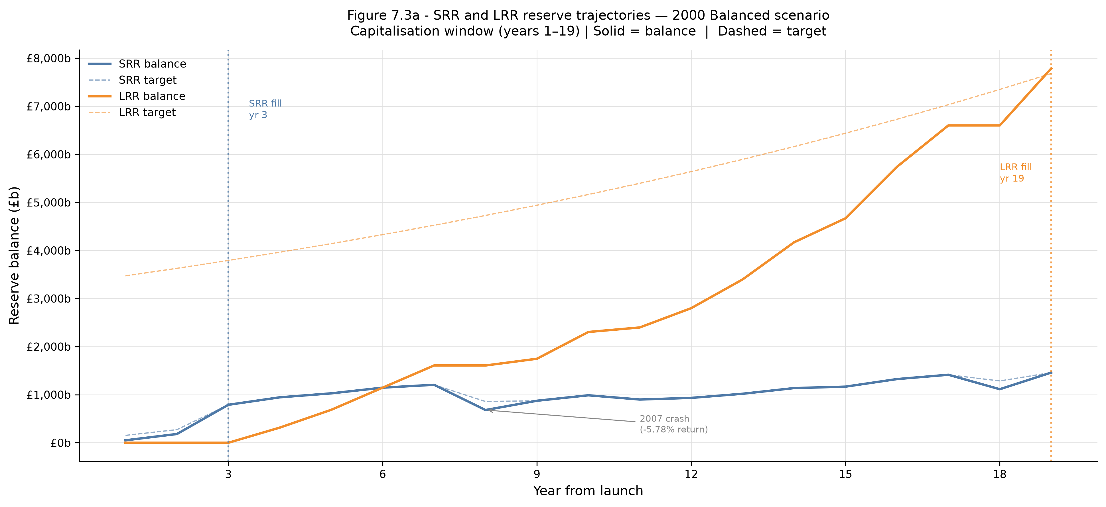
The SRR convergence reflects the reserve’s sizing logic: calibrated to net income under normal conditions, it fills quickly because early-year income, even in adverse sequences, is sufficient to reach the 3× floor. The LRR divergence reflects the cumulative effect of early-year return sequences on the accumulation trajectory from zero. The LRR balance crossing the LRR target line at year 19 is LRR fill, not overshoot: the target itself is growing throughout the window (3× annual expenditure, compounding at 4.51% p.a.), so crossing it requires the LRR balance to keep pace with a rising hurdle while accumulating from zero. That the balance slightly exceeds the target at fill reflects the LRR surplus of £104b recorded in (RATES.A §B.2) — the thinnest surplus of the crisis-decade starts, consistent with the 2000 scenario’s designation as the hardest illustrative case.
SRR fill signals that the refund guarantee is credible and that the economic case for modest tax relief has a reserve-backed foundation. LRR fill signals that fiscal replacement is viable. As noted in (RATES §6.3), whether and when the Governing Council acts on either signal is a political decision; Phase One and Phase Two are political operating postures, not labels for the intervals between economic milestones. At the 2000 reference scenario, SRR fill arrives at year 3 and LRR fill at year 19; under median starting conditions, LRR fill arrives at year 13.
7.4 Route D Deferred Revenue and Capitalisation Window Timing
The TCM models all taxpayers as generating annual delta revenue in each assessment period. This is correct for Routes A, B, and C, where the declared delta produces an annual tax liability or refund. It is not correct for Route D, where all settlement defers to a realisation event (a sale, death, or inheritance trigger) and no annual revenue flows until that event occurs.
Route D revenue is not lost; it is deferred. A Route D taxpayer who holds a position for twenty years and realises at year twenty contributes nothing to SRR or LRR fill in years one through nineteen and a potentially large lump sum in year twenty. The relevant question is how much Route D revenue falls within the capitalisation window rather than after it.
Annual realisation flows from the Route D population are estimable from three existing sources without live WDT data: ONS mortality data cross-referenced with the upper-tail wealth distribution (deaths trigger inheritance settlement); HMRC transaction data on private company sales and commercial property disposals (the principal Route D asset classes); and the inheritance and estate settlement record. That exercise has not been conducted here; it is a pre-Phase-One analytical deliverable added to the open questions register as item #33.
Pending that estimate, the RATES fill timelines should be understood as upper bounds on capitalisation speed. The degree of overstatement is proportional to the share of Route D wealth that does not realise within the capitalisation window. To bound the exposure: if Route D accounts for 20% of WDT-taxable wealth at the upper tail (the top of BEHAV.A §A.5’s estimated range) and no Route D position realised within the first thirty years of WDT operation, the revenue shortfall relative to the TCM baseline would be approximately 20% of the upper-tail contribution during that period, recovered in full at realisation thereafter. That scenario requires the simultaneous non-realisation of every Route D position across three decades, which is inconsistent with observed mortality rates and private asset transaction frequencies. The realistic impact is materially smaller and concentrated in the early capitalisation years, where the SRR’s 3× net revenue target provides the relevant buffer.
The SRR’s year-3 fill invariance result is robust to Route D deferrals by construction: the target is expressed as 3× observed net annual WDT revenue, so if deferrals reduce the annual revenue stream the target scales down proportionally and the fill timeline remains approximately three years regardless.
The LRR is different. The LRR floor is fixed in real terms (expressed as years of government expenditure, not as a multiple of observed revenue) and does not scale with the annual revenue stream. A sustained Route D deferral effect would extend the LRR breakeven year beyond the RATES §7.2 figures by a margin proportional to the revenue shortfall during the capitalisation window. Item #33 is designed to establish whether that extension is material. Given observed mortality rates and private asset transaction frequencies, the realistic effect is concentrated in the early capitalisation years and is unlikely to approach the theoretical upper bound of a 20% sustained revenue reduction across the full window.
7.4 Revenue Under the Predicted Declaration Distribution**
The TCM assumes \(\alpha\) = 1 throughout: every taxpayer declares their assets at true value in every assessment period. The behavioural analysis in (VAL §7), (VAL.A §A.6), and (ENV §2) predicts a population centre modestly above honest declaration, driven by refund-protection asymmetry under valuation uncertainty. (SWEEPS §11) establishes that mechanism intensity varies with wealth level. No paper in the series computes revenue under a population-weighted declaration distribution. This section addresses that omission.
The revenue consequences of departure from \(\alpha\) = 1 are asymmetric in a specific way. Systematic understatement (\(\alpha\) < 1) produces higher revenue than the baseline, not lower. An understating taxpayer declares a basis below true value; the basis gap compounds against them as the asset grows; the deferred liability recovers in full at realisation at the applicable marginal rate, which is higher than the rate that would have applied to the smoothed annual delta. The state collects more from a systematic understater than from an honest declarer on the same asset.
Systematic overstatement (\(\alpha\) > 1) also produces higher revenue during the accumulation period. A population centred at \(\alpha\) = 1.1 declares a tax base modestly above true values; annual deltas are correspondingly larger; the state collects slightly more than the honest-declaration baseline in each gain year. The RATES pre-behavioural revenue figures are therefore conservative with respect to the declaration distribution in the same direction as every other modelling assumption: actual declared revenue under any plausible declaration distribution is modestly higher than the TCM baseline.
The one scenario in which the declaration distribution creates a genuine risk is coordinated mass refund timing. If the population systematically overstates long enough to accumulate large lifetime envelope balances, and then coordinates maximum refund claims to fall in the same assessment year, the SRR faces a transient liquidity demand materially above its normal sizing. This is the declaration distribution’s worst case for the state: not a revenue shortfall, but a timing mismatch between accumulated refund entitlements and available SRR reserves.
Three structural features bound this risk. The lifetime contribution envelope caps each taxpayer’s refund entitlement at their cumulative prior contributions, so the mechanism cannot return more than it has collected from any individual regardless of declared loss size. The SRR is sized against a realistic refund exposure derived from the historical return series, not against the theoretical maximum of simultaneous full-envelope drawdown across the entire population. And the coordination requirement is itself a significant barrier: achieving a population-level timing event requires thousands of taxpayers and their professional advisers to simultaneously engineer large declared losses in the same assessment year. The population most capable of attempting this is also the population whose behaviour is most visible to the Administrator through the route distribution and declared value records, and whose coordinated action would constitute the egregious outlier pattern the corrective Route D auction pathway and Tier 1 monitoring are designed to detect.
The \(\alpha\) = 1 assumption in the TCM is conservative in both directions that matter for the revenue claims: systematic understatement and systematic overstatement both produce higher annual revenue than the baseline. The coordinated mass refund scenario is the only declaration-distribution outcome that creates a genuine SRR risk, and it is bounded by the envelope cap, the SRR’s reserve sizing, and the coordination barriers inherent in a dispersed population. The net effect of relaxing the \(\alpha\) = 1 assumption in the direction the behavioural analysis predicts is modestly higher revenue and a modestly faster LRR fill. A population-weighted revenue calculation across the predicted \(\alpha\) distribution — using the existing model infrastructure and the RATES bracket populations — is a natural analytical extension assigned to item #34 in the open questions register, and would confirm the direction of this argument with specific figures.
8. What Is Not in the Central Claim
8.1 The Corporate Levy
The corporate delta levy on listed companies is a designed component of the full WDT architecture (CORP §5). It is excluded from the reference revenue model because the attribution infrastructure required to implement it does not yet exist; including a speculative component would weaken rather than strengthen the reference claim. It is preserved here as quantified upside.
The calculation uses UK market capitalisation of £4.1 trillion and average annual market growth of 8.68%, giving an annual delta of approximately £356b. At 30% unattributable ownership and \(\tau_c\) = \(\tau_m\) = 70%, the reference estimate is £172b. The attribution sensitivity is as follows.
| Unattributable % | Identifiable and attributable (£b) | Attrib. not identified (£b) | Unattributable (£b) | Total (£b) |
|---|---|---|---|---|
| 20% | £0 | £82 | £60 | £142 |
| 30% | £0 | £82 | £90 | £172 |
| 40% | £0 | £82 | £120 | £202 |
| 50% | £0 | £82 | £150 | £232 |
| 60% | £0 | £82 | £180 | £262 |
| 70% | £0 | £82 | £210 | £292 |
| 80% | £0 | £82 | £240 | £322 |
The identifiable and attributable tranche reconciles entirely through the individual WDT mechanism; net corporate levy revenue from that tranche is zero. The attributable-but-not-identified tranche is held at approximately 10% of market capitalisation (£82b) across all rows at \(\tau_c\) = \(\tau_m\) = 70%.
The additivity of the corporate levy estimate and the individual WDT figure of £874b follows directly from the table. The only population that could produce double-counting (native WDT shareholders whose listed equity is already included in their declared net worth) contributes zero net corporate levy revenue, because the provisional levy on that tranche is released in full on individual settlement. The £172b reference estimate derives entirely from beneficial owners who have no individual WDT assessment position, whose wealth is therefore not captured in the TCM’s £874b figure, and whose market capitalisation delta is incremental revenue rather than a duplicate collection.
The range of £142b–£322b broadly matches the UK corporate tax cluster of approximately £213.5b in 2022–23. The revenue estimate uses \(\tau_c\) = \(\tau_m\) = 70% as the working ceiling assumption for the unattributable tranche, representing the ceiling of the plausible range as established in (CORP.A §B.2). That section derives the appropriate range for \(\tau_h\) from competing objectives (deterrence of deliberate opacity, revenue recovery, the partial deterrence provided by forfeiture of refund rights, and legal proportionality in the absence of individual assessment) and concludes that \(\tau_m\) is a defensible ceiling rather than a settled anchor. Exact calibration within the range above \(\tau_0\) and at or below \(\tau_m\) remains a Governing Council parameter informed by Phase One evidence and jurisdiction-specific legal analysis.
8.2 The Ultra-High-Net-Worth Tail
The Pareto model’s practical upper bound of approximately £140m lies far below the actual holdings of the UK’s wealthiest individuals (the largest Sunday Times Rich List entry at approximately £20.9b is roughly 150 times the ceiling). The gap is addressed separately rather than incorporated into the reference estimate because this population is the most capable of international mobility and restructuring; including them without modelling behavioural response would overstate revenue in exactly the bracket where overstatement is most plausible.
The bespoke calculation uses the 55 wealthiest UK individuals with combined estimated net worth of £273.4b. At 8.3% annual growth and an effective rate of approximately 69.9% of the \(\tau_m\) ceiling, the annual contribution is approximately £27b, likely a floor since public wealth estimates for this population are typically conservative. If all 55 departed before the WDT came into force, the core individual WDT claim is unaffected.
8.3 Combined Pre-Behavioural Estimate
The three components can be assembled into a conservative combined ceiling, even though each carries its own uncertainty and none is modelled to the same standard as the individual WDT reference.
| Component | Annual estimate | Basis |
|---|---|---|
| Individual WDT (lifetime avg, N=30) | £873.6b | TCM, 2000 scenario, Balanced parameters |
| Corporate delta levy | £172b | 30% unattributable; \(\tau_c\) = \(\tau_m\) = 70% |
| UHNW tail (top 55) | £27b | Bespoke calculation; public wealth estimates |
| Combined pre-behavioural ceiling | ~£1,073b | Sum of above; components are additive pre-behaviour |
Against a UK government expenditure base of £1,157b in 2022–23 (JUR §3.2), a pre-behavioural combined estimate of approximately £1,073b represents near-parity with current total managed expenditure — at a calibration chosen specifically to represent the worst historical starting conditions and with individual burdens that remain proportionate throughout. This figure should not be treated as a revenue forecast. Behavioural responses will reduce it, the components share uncertainty of different kinds, and the corporate and UHNW figures use ceiling assumptions. The purpose of the combined estimate is narrower: to establish that the central individual WDT claim, already demonstrated as arithmetically sound under the hardest historical conditions, substantially understates the mechanism’s full fiscal capacity. The burden of proof does not rest with demonstrating that the WDT can raise enough revenue; it rests with demonstrating that behavioural responses reduce it below the level where fiscal replacement remains viable.
9. Limitations and Further Work
9.1 Formal modelling gaps
The revenue model is built on a fixed historical UK equity return series as a growth proxy for broad wealth across asset classes. This is the best available single series but reflects one country over one period (1947–2019). A different national return series, finer-grained data, or a longer historical record would produce different sweep figures. A formal cross-country or cross-period analysis of the model’s sensitivity to the choice of return series has not been done.
The formal welfare comparisons that this paper’s burden figures implied but did not carry out — comparing the WDT against capital gains tax, income tax on capital, a stock wealth tax, a consumption tax, and an accrual tax at genuine revenue equivalence — have since been undertaken in (WFR §3) and (WFR §4). The Domar-Musgrave extension to a progressive delta base, identified as a gap in (LR.A §2.1), is addressed in (WFR §3.2) and (WFR §4.1). The distributional concentration arithmetic across a four-tier Fagereng calibration, identified as a gap in (LR.A §2.3), is in (WFR §4.3).
9.2 Phase One empirical unknowns
The revenue estimates are explicitly pre-behavioural. Migration, restructuring, and avoidance will reduce actual revenue by an unknown amount. The pre-behavioural figures should be treated as an upper-bound starting point, not an expected outcome. Complete behavioural modelling — migration, restructuring, avoidance, and the cross-base externality during Phase One — is the principal outstanding analytical task before a post-response revenue estimate can be made.
The cross-base externality (Agrawal et al., 2025) — income tax and VAT losses approximately six times larger than the direct wealth-tax revenue loss — applies during Phase One when existing taxes operate alongside the WDT pilot. In Phase Two, where the WDT’s revenue displaces those parallel taxes, the externality disappears structurally. The Phase One exposure is unresolved. BEHAV sets out the design framework within which Phase One can generate evidence on it.
Phase One transition costs — compliance infrastructure, institutional capacity build-out, and the coexistence of WDT and existing taxes — are not modelled. They are partly Phase One empirical questions and partly addressed by the implementation pathway in (WP §7).
9.3 Jurisdiction-specific legal and implementation work
No items in this paper beyond those inherited from CORP (CIT interaction, #31) and GOV (Governing Council milestone declaration criteria).
9.4 Structural and irreducible limits of the design
The TCM’s persistent heterogeneous growth tier differentials are a stylisation. The SSM applies historical equity returns uniformly across the entire taxable population as the worst-case correlated-shock assumption. Neither is the true model of how wealth grows across asset classes and individuals. A return sequence worse than any observed in the 1947–2019 UK data would extend the LRR breakeven beyond the 29-year worst case in the historical sweep (2006 and 2007 start years) and would likely depress post-fill coverage further below the 2000 reference minimum; the paper does not claim robustness beyond the historical range.
The paper does not model the political economy of the transition. The Governing Council’s ability to commit to a chosen calibration across electoral cycles depends on political conditions beyond this analysis.
The fill timelines assume canonical parameters held constant across the capitalisation window. Governing Council rate decisions are modelled as exogenous: the TCM does not simulate how chamber dynamics might alter parameters over time. TP’s rational preference for lower τ₀, combined with potential near-threshold member dominance as the enrolled population grows, could produce persistent downward rate pressure that extends the LRR fill timeline beyond the figures in §7.2. The τ₀ × W_min joint surface (open questions register item #17) characterises the fill timeline’s sensitivity to τ₀ reduction and should be completed before Phase One begins.
9.5 Governing Council calibration parameters
The formal criteria by which the Governing Council declares SRR fill achieved and initiates first-phase tax relief, and the corresponding criteria for declaring LRR fill and commencing full Phase Two, are Tier 1 process parameters. This paper establishes when each milestone is reached; how that moment translates into specific political decisions is a Governing Council matter.
Once the LRR meets its floor target, the governance architecture requires rate review. The direction is clear — rates fall or the threshold rises, redirecting surplus toward the labour tax relief dividend — but the specific recalibration is a Governing Council decision informed by Phase One behavioural data and the prevailing SRR capitalisation ratio at the time.
10. Conclusion
The arithmetic works, and it works without exception across the full range of historical starting conditions the mechanism might inherit.
The historical starting-year sweep produces a 100% success rate under the v8 success definition across all 73 start years and all four economic cycles. Success is defined precisely: the LRR fills within the 71-year modelling window and the LRR never fails. The mechanism does not fail under any historical return sequence available. No start year produces an LRR or SRR failure.
Two robustness properties hold on different timescales. The SRR fill year is invariant at 3 across all 73 start years: the refund guarantee becomes mechanically credible within 3 years regardless of starting conditions. The LRR breakeven ranges from 7 to 29 years, with a median of 13. The 2000 reference scenario — chosen because it produces the lowest 10-year post-fill TCM coverage in the sweep — fills at year 19. Individual WDT revenue alone meets the fiscal target in every case. The corporate levy and ultra-high-net-worth tail supplement sit above these figures as unmodelled upside. Phase One is self-financing at the reference calibration.
At the 2000 Balanced reference, the population-weighted average annual wealth burden across all modelled taxpayers is 0.24% of net worth per year; the revenue-weighted average is 0.35%. Both figures sit well below the 1–2% annual stock levy of most proposed wealth taxes — the WDT’s delta base produces structurally lighter annual charges than any equivalent stock-based mechanism at the same revenue scale. The maximum annual wealth burden is 0.79% of net worth per year, a ceiling requiring simultaneous membership of the top 0.01% wealth bracket and the highest persistent-outperformance growth tier across the canonical 30-year burden horizon. For most taxpayers the annual cost is a fraction of a percent of existing wealth: the tax base is the annual increment, and the symmetric refund mechanism means loss years offset gain years over the lifetime horizon.
The gain-weighted effective rate on lifetime gains is 13.0% — total WDT collected as a fraction of total lifetime wealth increase across the modelled population, directly comparable to a statutory CGT or income tax rate applied to aggregate gains. The maximum effective rate of 27.2% sits at the very top of both distributions simultaneously, as a lifetime average over 30 years that includes both gain years and loss years with refunds. Across the broad body of the distribution the effective rate ranges from zero (lower brackets in below-average growth tiers, where refunds in loss years offset gain-year liabilities) to the mid-teens, rising with both wealth level and growth experience. The mechanism taxes persistent outperformance compounding at scale; it does not tax wealth that fails to grow.
The labour tax relief dividend becomes viable at LRR fill — year 19 under the 2000 reference scenario, year 13 under median starting conditions. In the first 10 years after LRR fill, the mechanism delivers Step-5 labour-relief surplus equivalent to 6.4% (SSM floor) to 14.6% (TCM ceiling) of government expenditure at the 2000 reference, and 125.5% (TCM median) across the full sweep. The SRR fills at year 3 under any historical starting conditions, marking the moment the refund guarantee is credible and the case for incremental tax relief has a reserve-backed foundation. The transition timescale is what the Governing Council monitors as the primary indicator of progress; Phase One and Phase Two are political operating postures it controls, not labels for the intervals between economic milestones.
This paper has established four properties of the WDT simultaneously, at a calibration chosen to represent the hardest historical starting conditions available. First, the mechanism eliminates the stock-versus-flow problem by taxing the annual delta: the revenue-weighted annual burden of 0.35% is structurally lighter than any stock-based wealth tax at comparable revenue scale, because wealth that does not grow is not taxed. Second, the symmetric refund guarantee becomes mechanically credible within a single political cycle — three years — under every historical return sequence in the dataset, including sequences that front-load severe crashes. Third, the mechanism delivers meaningful fiscal replacement capacity across all 73 historical starting conditions without exception: the LRR fills and never fails in every case, and the post-fill surplus exceeds 14% of government expenditure at the hardest start and 125% at the median. Fourth, it does so at individual burdens that are proportionate by any conventional standard: the gain-weighted effective rate on lifetime gains of 13.0% compares favourably to statutory CGT rates on a materially larger base, including gains that current tax law never reaches.
No prior wealth tax proposal has satisfied all four properties simultaneously. The standard failure modes — exhausting the capital base, creating insupportable refund liabilities in crash years, concentrating transition risk on favourable starting conditions, or imposing burdens disproportionate to gains realised — are each addressed by features of the mechanism that reinforce rather than trade off against each other. This paper has not shown that the WDT will succeed in practice; behavioural responses, political economy, and implementation complexity remain unresolved. What it has shown is that there is no arithmetic or structural reason for it to fail. The burden of proof now sits with those who claim otherwise.